Volatility Forecasting
This setup code is required to run in an IPython notebook
[1]:
import warnings
warnings.simplefilter('ignore')

%matplotlib inline
import matplotlib.pyplot as plt
import seaborn as sns

sns.set_style('darkgrid')
plt.rc("figure", figsize=(16, 6))
plt.rc("savefig", dpi=90)
plt.rc("font",family="sans-serif")
plt.rc("font",size=14)
Data
These examples make use of S&P 500 data from Yahoo! that is available from arch.data.sp500.
[2]:
import datetime as dt
import sys

import numpy as np
import pandas as pd

from arch import arch_model
import arch.data.sp500

data = arch.data.sp500.load()
market = data['Adj Close']
returns = 100 * market.pct_change().dropna()
Basic Forecasting
Forecasts can be generated for standard GARCH(p,q) processes using any of the three forecast generation methods:
Analytical
Simulation-based
Bootstrap-based
Be default forecasts will only be produced for the final observation in the sample so that they are out-of-sample.
Forecasts start with specifying the model and estimating parameters.
[3]:
am = arch_model(returns, vol='Garch', p=1, o=0, q=1, dist='Normal')
res = am.fit(update_freq=5)
Iteration:      5,   Func. Count:     39,   Neg. LLF: 6942.159596737265
Iteration:     10,   Func. Count:     72,   Neg. LLF: 6936.718529994181
Optimization terminated successfully.    (Exit mode 0)
            Current function value: 6936.718476989043
            Iterations: 11
            Function evaluations: 79
            Gradient evaluations: 11
[4]:
forecasts = res.forecast()
Forecasts are contained in an ARCHModelForecast object which has 4 attributes:
mean- The forecast meansresidual_variance- The forecast residual variances, that is \(E_t[\epsilon_{t+h}^2]\)variance- The forecast variance of the process, \(E_t[r_{t+h}^2]\). The variance will differ from the residual variance whenever the model has mean dynamics, e.g., in an AR process.simulations- An object that contains detailed information about the simulations used to generate forecasts. Only used if the forecastmethodis set to'simulation'or'bootstrap'. If using'analytical'(the default), this isNone.
The three main outputs are all returned in DataFrames with columns of the form h.# where # is the number of steps ahead. That is, h.1 corresponds to one-step ahead forecasts while h.10 corresponds to 10-steps ahead.
The default forecast only produces 1-step ahead forecasts.
[5]:
print(forecasts.mean.iloc[-3:])
print(forecasts.residual_variance.iloc[-3:])
print(forecasts.variance.iloc[-3:])
                 h.1
Date
2018-12-27       NaN
2018-12-28       NaN
2018-12-31  0.056353
                h.1
Date
2018-12-27      NaN
2018-12-28      NaN
2018-12-31  3.59647
                h.1
Date
2018-12-27      NaN
2018-12-28      NaN
2018-12-31  3.59647
Longer horizon forecasts can be computed by passing the parameter horizon.
[6]:
forecasts = res.forecast(horizon=5)
print(forecasts.residual_variance.iloc[-3:])
                h.1       h.2       h.3       h.4     h.5
Date
2018-12-27      NaN       NaN       NaN       NaN     NaN
2018-12-28      NaN       NaN       NaN       NaN     NaN
2018-12-31  3.59647  3.568502  3.540887  3.513621  3.4867
Values that are not computed are nan-filled.
Alternative Forecast Generation Schemes
Fixed Window Forecasting
Fixed-windows forecasting uses data up to a specified date to generate all forecasts after that date. This can be implemented by passing the entire data in when initializing the model and then using last_obs when calling fit. forecast() will, by default, produce forecasts after this final date.
Note last_obs follow Python sequence rules so that the actual date in last_obs is not in the sample.
[7]:
res = am.fit(last_obs='2011-1-1', update_freq=5)
forecasts = res.forecast(horizon=5)
print(forecasts.variance.dropna().head())
Iteration:      5,   Func. Count:     38,   Neg. LLF: 4559.84602040562
Iteration:     10,   Func. Count:     72,   Neg. LLF: 4555.383725179201
Optimization terminated successfully.    (Exit mode 0)
            Current function value: 4555.285110045353
            Iterations: 14
            Function evaluations: 97
            Gradient evaluations: 14
                 h.1       h.2       h.3       h.4       h.5
Date
2010-12-31  0.381757  0.390905  0.399988  0.409008  0.417964
2011-01-03  0.451724  0.460381  0.468976  0.477512  0.485987
2011-01-04  0.428416  0.437236  0.445994  0.454691  0.463326
2011-01-05  0.420554  0.429429  0.438242  0.446993  0.455683
2011-01-06  0.402483  0.411486  0.420425  0.429301  0.438115
Rolling Window Forecasting
Rolling window forecasts use a fixed sample length and then produce one-step from the final observation. These can be implemented using first_obs and last_obs.
[8]:
index = returns.index
start_loc = 0
end_loc = np.where(index >= '2010-1-1')[0].min()
forecasts = {}
for i in range(20):
    sys.stdout.write('.')
    sys.stdout.flush()
    res = am.fit(first_obs=i, last_obs=i + end_loc, disp='off')
    temp = res.forecast(horizon=3).variance
    fcast = temp.iloc[i + end_loc - 1]
    forecasts[fcast.name] = fcast
print()
print(pd.DataFrame(forecasts).T)
....................
                 h.1       h.2       h.3
2009-12-31  0.615314  0.621743  0.628133
2010-01-04  0.751747  0.757343  0.762905
2010-01-05  0.710453  0.716315  0.722142
2010-01-06  0.666244  0.672346  0.678411
2010-01-07  0.634424  0.640706  0.646949
2010-01-08  0.600109  0.606595  0.613040
2010-01-11  0.565514  0.572212  0.578869
2010-01-12  0.599561  0.606051  0.612501
2010-01-13  0.608309  0.614748  0.621148
2010-01-14  0.575065  0.581756  0.588406
2010-01-15  0.629890  0.636245  0.642561
2010-01-19  0.695074  0.701042  0.706974
2010-01-20  0.737154  0.742908  0.748627
2010-01-21  0.954167  0.958725  0.963255
2010-01-22  1.253453  1.256401  1.259332
2010-01-25  1.178691  1.182043  1.185374
2010-01-26  1.112205  1.115886  1.119545
2010-01-27  1.051295  1.055327  1.059335
2010-01-28  1.085678  1.089512  1.093324
2010-01-29  1.085786  1.089593  1.093378
Recursive Forecast Generation
Recursive is similar to rolling except that the initial observation does not change. This can be easily implemented by dropping the first_obs input.
[9]:
import numpy as np
import pandas as pd

index = returns.index
start_loc = 0
end_loc = np.where(index >= '2010-1-1')[0].min()
forecasts = {}
for i in range(20):
    sys.stdout.write('.')
    sys.stdout.flush()
    res = am.fit(last_obs=i + end_loc, disp='off')
    temp = res.forecast(horizon=3).variance
    fcast = temp.iloc[i + end_loc - 1]
    forecasts[fcast.name] = fcast
print()
print(pd.DataFrame(forecasts).T)
....................
                 h.1       h.2       h.3
2009-12-31  0.615314  0.621743  0.628133
2010-01-04  0.751723  0.757321  0.762885
2010-01-05  0.709956  0.715791  0.721591
2010-01-06  0.666057  0.672146  0.678197
2010-01-07  0.634503  0.640776  0.647011
2010-01-08  0.600417  0.606893  0.613329
2010-01-11  0.565684  0.572369  0.579014
2010-01-12  0.599963  0.606438  0.612874
2010-01-13  0.608558  0.614982  0.621366
2010-01-14  0.575020  0.581639  0.588217
2010-01-15  0.629696  0.635989  0.642244
2010-01-19  0.694735  0.700656  0.706541
2010-01-20  0.736509  0.742193  0.747842
2010-01-21  0.952751  0.957245  0.961713
2010-01-22  1.251145  1.254050  1.256936
2010-01-25  1.176864  1.180162  1.183441
2010-01-26  1.110848  1.114497  1.118124
2010-01-27  1.050102  1.054077  1.058028
2010-01-28  1.084669  1.088454  1.092216
2010-01-29  1.085003  1.088783  1.092541
TARCH
Analytical Forecasts
All ARCH-type models have one-step analytical forecasts. Longer horizons only have closed forms for specific models. TARCH models do not have closed-form (analytical) forecasts for horizons larger than 1, and so simulation or bootstrapping is required. Attempting to produce forecasts for horizons larger than 1 using method='analytical' results in a ValueError.
[10]:
# TARCH specification
am = arch_model(returns, vol='GARCH', power=2.0, p=1, o=1, q=1)
res = am.fit(update_freq=5)
forecasts = res.forecast()
print(forecasts.variance.iloc[-1])
Iteration:      5,   Func. Count:     44,   Neg. LLF: 6827.96641441215
Iteration:     10,   Func. Count:     84,   Neg. LLF: 6822.8830945206155
Optimization terminated successfully.    (Exit mode 0)
            Current function value: 6822.882823359995
            Iterations: 13
            Function evaluations: 106
            Gradient evaluations: 13
h.1    3.010188
Name: 2018-12-31 00:00:00, dtype: float64
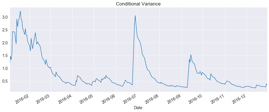
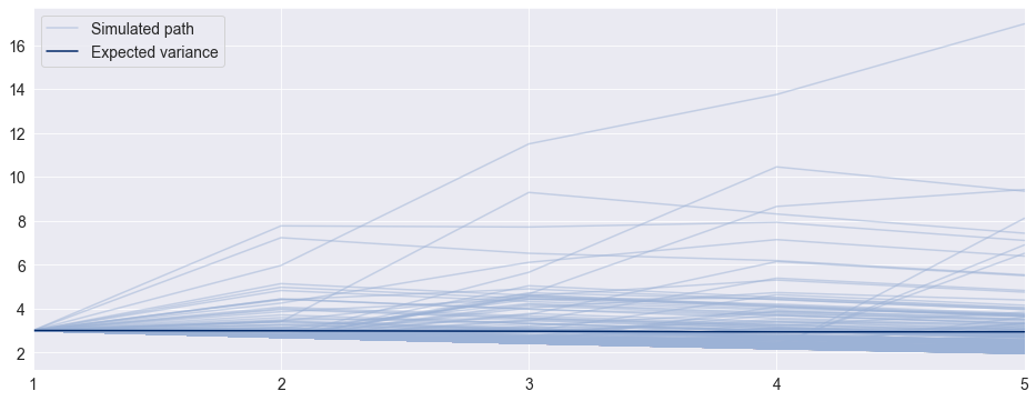
Simulation Forecasts
When using simulation- or bootstrap-based forecasts, an additional attribute of an ARCHModelForecast object is meaningful -- simulation.
[11]:
import matplotlib.pyplot as plt
fig, ax = plt.subplots(1, 1)
var_2016 = res.conditional_volatility['2016']**2.0
subplot = var_2016.plot(ax=ax, title='Conditional Variance')
subplot.set_xlim(var_2016.index[0], var_2016.index[-1])
[11]:
(735967.0, 736328.0)
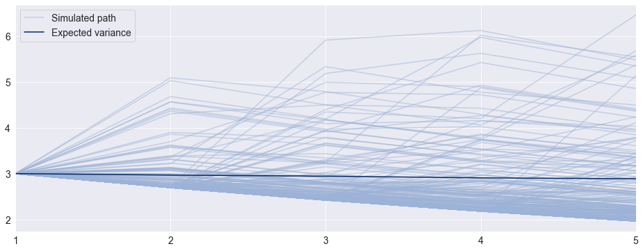
[12]:
forecasts = res.forecast(horizon=5, method='simulation')
sims = forecasts.simulations

x = np.arange(1, 6)
lines = plt.plot(x, sims.residual_variances[-1, ::5].T, color='#9cb2d6', alpha=0.5)
lines[0].set_label('Simulated path')
line = plt.plot(x, forecasts.variance.iloc[-1].values, color='#002868')
line[0].set_label('Expected variance')
plt.gca().set_xticks(x)
plt.gca().set_xlim(1,5)
legend = plt.legend()
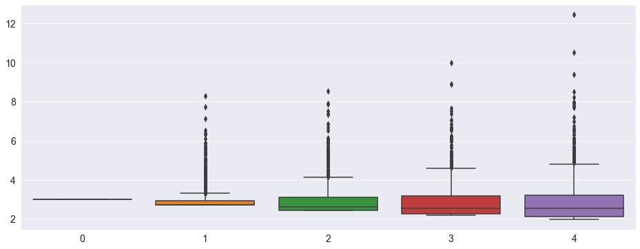
[13]:
import seaborn as sns
sns.boxplot(data=sims.variances[-1])
[13]:
<matplotlib.axes._subplots.AxesSubplot at 0x29d80214388>
Bootstrap Forecasts
Bootstrap-based forecasts are nearly identical to simulation-based forecasts except that the values used to simulate the process are computed from historical data rather than using the assumed distribution of the residuals. Forecasts produced using this method also return an ARCHModelForecastSimulation containing information about the simulated paths.
[14]:
forecasts = res.forecast(horizon=5, method='bootstrap')
sims = forecasts.simulations

lines = plt.plot(x, sims.residual_variances[-1, ::5].T, color='#9cb2d6', alpha=0.5)
lines[0].set_label('Simulated path')
line = plt.plot(x, forecasts.variance.iloc[-1].values, color='#002868')
line[0].set_label('Expected variance')
plt.gca().set_xticks(x)
plt.gca().set_xlim(1,5)
legend = plt.legend()
Value-at-Risk Forecasting
Value-at-Risk (VaR) forecasts from GARCH models depend on the conditional mean, the conditional volatility and the quantile of the standardized residuals,
where \(q_{\alpha}\) is the \(\alpha\) quantile of the standardized residuals, e.g., 5%.
The quantile can be either computed from the estimated model density or computed using the empirical distribution of the standardized residuals. The example below shows both methods.
[15]:
am = arch_model(returns, vol='Garch', p=1, o=0, q=1, dist='skewt')
res = am.fit(disp='off', last_obs='2017-12-31')
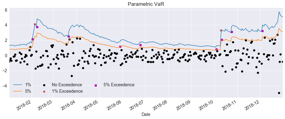
Parametric VaR
First, we use the model to estimate the VaR. The quantiles can be computed using the ppf method of the distribution attached to the model. The quantiles are printed below.
[16]:
forecasts = res.forecast(start='2018-1-1')
cond_mean = forecasts.mean['2018':]
cond_var = forecasts.variance['2018':]
q = am.distribution.ppf([0.01, 0.05], res.params[-2:])
print(q)
[-2.64485046 -1.64965888]
Next, we plot the two VaRs along with the returns. The returns that violate the VaR forecasts are highlighted.
[17]:
value_at_risk = -cond_mean.values - np.sqrt(cond_var).values * q[None, :]
value_at_risk = pd.DataFrame(
    value_at_risk, columns=['1%', '5%'], index=cond_var.index)
ax = value_at_risk.plot(legend=False)
xl = ax.set_xlim(value_at_risk.index[0], value_at_risk.index[-1])
rets_2018 = returns['2018':].copy()
rets_2018.name = 'S&P 500 Return'
c = []
for idx in value_at_risk.index:
    if rets_2018[idx] > -value_at_risk.loc[idx, '5%']:
        c.append('#000000')
    elif rets_2018[idx] < -value_at_risk.loc[idx, '1%']:
        c.append('#BB0000')
    else:
        c.append('#BB00BB')
c = np.array(c, dtype='object')
labels = {
    '#BB0000': '1% Exceedence',
    '#BB00BB': '5% Exceedence',
    '#000000': 'No Exceedence'
}
markers = {'#BB0000': 'x', '#BB00BB': 's', '#000000': 'o'}
for color in np.unique(c):
    sel = c == color
    ax.scatter(
        rets_2018.index[sel],
        -rets_2018.loc[sel],
        marker=markers[color],
        c=c[sel],
        label=labels[color])
ax.set_title('Parametric VaR')
leg = ax.legend(frameon=False, ncol=3)
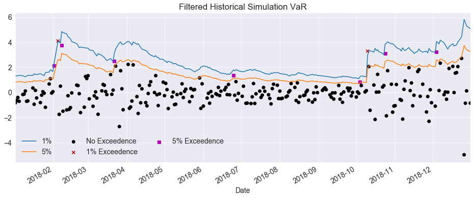
Filtered Historical Simulation
Next, we use the empirical distribution of the standardized residuals to estimate the quantiles. These values are very similar to those estimated using the assumed distribution. The plot below is identical except for the slightly different quantiles.
[18]:
std_rets = (returns[:'2017'] - res.params['mu']) / res.conditional_volatility
std_rets = std_rets.dropna()
q = std_rets.quantile([.01, .05])
print(q)
0.01   -2.668272
0.05   -1.723352
dtype: float64
[19]:
value_at_risk = -cond_mean.values - np.sqrt(cond_var).values * q.values[None, :]
value_at_risk = pd.DataFrame(
    value_at_risk, columns=['1%', '5%'], index=cond_var.index)
ax = value_at_risk.plot(legend=False)
xl = ax.set_xlim(value_at_risk.index[0], value_at_risk.index[-1])
rets_2018 = returns['2018':].copy()
rets_2018.name = 'S&P 500 Return'
c = []
for idx in value_at_risk.index:
    if rets_2018[idx] > -value_at_risk.loc[idx, '5%']:
        c.append('#000000')
    elif rets_2018[idx] < -value_at_risk.loc[idx, '1%']:
        c.append('#BB0000')
    else:
        c.append('#BB00BB')
c = np.array(c, dtype='object')
for color in np.unique(c):
    sel = c == color
    ax.scatter(
        rets_2018.index[sel],
        -rets_2018.loc[sel],
        marker=markers[color],
        c=c[sel],
        label=labels[color])
ax.set_title('Filtered Historical Simulation VaR')
leg = ax.legend(frameon=False, ncol=3)