Examples
System regression simultaneously estimates multiple models. This has three distinct advantages:
Joint inference across models
Linear restrictions can be imposed on the parameters across different models
Improved precision of parameter estimates (depending on the model specification and data)
There are \(K\) models and each model can be expressed in vector notation as
so that the set of models can be expressed as
where \(Y\) is a column vector that stacks the vectors \(Y_i\) for \(i=1,2,\ldots,K\), \(X\) is a block-diagonal matrix where diagonal block i is \(X_i\), \(\beta\) is a stacked vector of the \(K\) \(\beta_i\)s and \(\epsilon\) is similarly comprised of the stacked columns of \(\epsilon_i\).
The model can be estimated using OLS with the usual estimator
Since there are multiple series, a GLS estimator that accounts for the cross-sectional heteroskedasticity as well as the correlation of residuals can be estimated
where \(\Omega^{-1} = \Sigma^{-1} \otimes I_{T}\), \(\Sigma_{ij}\) is the covariance between \(\epsilon_i\) and \(\epsilon_j\) and \(T\) is the number of observations. The GLS estimator is only beneficial when the regressors in different models differ and when residuals are correlated. There GLS estimates are identical to the multivariate OLS estimates when all regressors are common.
[1]:
# Common libraries
import numpy as np
import pandas as pd
import seaborn as sns
import statsmodels.api as sm
Data
Two data sets will be used. The first is from Munnell which looks at the effect of capital on state GDP. This example follows the example in Chapter 10 in recent editions of Greene”s Econometric Analysis.
The data is state-level but the model is estimated in region. The first step is to aggregate the data by region. All capital measures are summed and the unemployment rate is averaged using weights proportional to the total employment in each state.
[2]:
from linearmodels.datasets import munnell

data = munnell.load()

regions = {
    "GF": ["AL", "FL", "LA", "MS"],
    "MW": ["IL", "IN", "KY", "MI", "MN", "OH", "WI"],
    "MA": ["DE", "MD", "NJ", "NY", "PA", "VA"],
    "MT": ["CO", "ID", "MT", "ND", "SD", "WY"],
    "NE": ["CT", "ME", "MA", "NH", "RI", "VT"],
    "SO": ["GA", "NC", "SC", "TN", "WV", "AR"],
    "SW": ["AZ", "NV", "NM", "TX", "UT"],
    "CN": ["AK", "IA", "KS", "MO", "NE", "OK"],
    "WC": ["CA", "OR", "WA"],
}


def map_region(state):
    for key in regions:
        if state in regions[key]:
            return key


data["REGION"] = data.ST_ABB.map(map_region)
data["TOTAL_EMP"] = data.groupby(["REGION", "YR"])["EMP"].transform("sum")
data["EMP_SHARE"] = data.EMP / data.TOTAL_EMP
data["WEIGHED_UNEMP"] = data.EMP_SHARE * data.UNEMP
A groupby transformation is used to aggregate the data, and finally all values except the unemployment rate are logged.
[3]:
grouped = data.groupby(["REGION", "YR"])
agg_data = grouped[["GSP", "PC", "HWY", "WATER", "UTIL", "EMP", "WEIGHED_UNEMP"]].sum()
for col in ["GSP", "PC", "HWY", "WATER", "UTIL", "EMP"]:
    agg_data["ln" + col] = np.log(agg_data[col])
agg_data["UNEMP"] = agg_data.WEIGHED_UNEMP
agg_data["Intercept"] = 1.0
Basic Usage
Seemingly Unrelated Models are fairly complex and each equation could have a different number of regressors. As a result, it is not possibly to use standard pandas or numpy data structures, and so dictionaries (or technically dictionary-like objects) are used. In practice, it is strongly recommended to use a OrderedDictionary from the collections module. This ensures that equation order will be preserved. In addition, the dictionary must have the following structure:
keysmust be strings and will be used as equation labelsThe value associated with each key must be either a dictionary or a tuple.
When a dictionary is used, it must have two keys,
dependentandexog. It can optionally have a third keyweightswhich provides weights to use in the regression.When a tuple is used, it must have two elements and takes the form
(dependent, exog). It can optionally contains weights in which case it takes the form(dependent, exog, weights).
This example uses the dictionary syntax to contain the data for each region and uses the region identified as the equation label.
[4]:
from collections import OrderedDict

mod_data = OrderedDict()
for region in ["GF", "SW", "WC", "MT", "NE", "MA", "SO", "MW", "CN"]:
    region_data = agg_data.loc[region]
    dependent = region_data.lnGSP
    exog = region_data[
        ["Intercept", "lnPC", "lnHWY", "lnWATER", "lnUTIL", "lnEMP", "UNEMP"]
    ]
    mod_data[region] = {"dependent": dependent, "exog": exog}
Fitting the model is virtually identical to fitting any other model with the exception of the special data structure required.
The fitting options here ensure that the homoskedastic covariance estimator are used (cov_type="unadjusted") and that a small sample adjustment is applied. By default, GLS is used (this can be overridden using method="ols".
[5]:
from linearmodels.system import SUR

mod = SUR(mod_data)
res = mod.fit(cov_type="unadjusted")
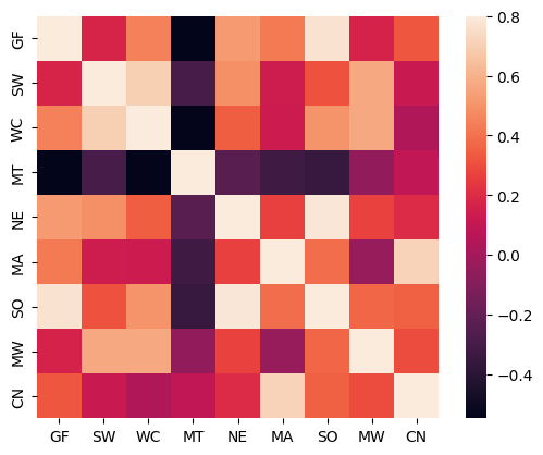
One of the requirements for there to be an efficiency gain in a SUR is that the residuals are correlated. A heatmap is used to inspect this correlation, which is substantial and varies by region.
[6]:
import matplotlib.pyplot as plt

cov = res.sigma
std = np.sqrt(np.diag(res.sigma)[:, None])
regions = list(mod_data.keys())
corr = pd.DataFrame(cov / (std @ std.T), columns=regions, index=regions)

sns.heatmap(corr, vmax=0.8, square=True)
plt.show()

corr.style.format("{:0.3f}")
[6]:
| GF | SW | WC | MT | NE | MA | SO | MW | CN | |
|---|---|---|---|---|---|---|---|---|---|
| GF | 1.000 | 0.173 | 0.447 | -0.547 | 0.525 | 0.425 | 0.763 | 0.167 | 0.325 |
| SW | 0.173 | 1.000 | 0.697 | -0.290 | 0.489 | 0.132 | 0.314 | 0.565 | 0.119 |
| WC | 0.447 | 0.697 | 1.000 | -0.537 | 0.343 | 0.130 | 0.505 | 0.574 | 0.037 |
| MT | -0.547 | -0.290 | -0.537 | 1.000 | -0.241 | -0.322 | -0.351 | -0.058 | 0.091 |
| NE | 0.525 | 0.489 | 0.343 | -0.241 | 1.000 | 0.259 | 0.783 | 0.269 | 0.200 |
| MA | 0.425 | 0.132 | 0.130 | -0.322 | 0.259 | 1.000 | 0.388 | -0.037 | 0.713 |
| SO | 0.763 | 0.314 | 0.505 | -0.351 | 0.783 | 0.388 | 1.000 | 0.366 | 0.350 |
| MW | 0.167 | 0.565 | 0.574 | -0.058 | 0.269 | -0.037 | 0.366 | 1.000 | 0.298 |
| CN | 0.325 | 0.119 | 0.037 | 0.091 | 0.200 | 0.713 | 0.350 | 0.298 | 1.000 |
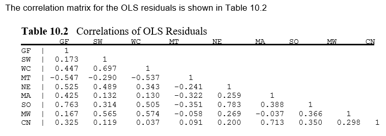
These values can be seen to be identical to the reported results in the existing example from Greene.
[7]:
from IPython.display import Image, display_png

display_png(Image("system_correct-greene-table-10-2.png"))
The full result is fairly long and so here I only print the first 33 lines which show results for two regions. By default it reports all estimates along with the usual measures of precision.
[8]:
print("\n".join(res.summary.as_text().split("\n")[:33]))
                           System GLS Estimation Summary
===================================================================================
Estimator:                        GLS   Overall R-squared:                   0.9937
No. Equations.:                     9   McElroy's R-squared:                 0.9988
No. Observations:                  17   Judge's (OLS) R-squared:             0.9937
Date:                Tue, Oct 21 2025   Berndt's R-squared:                  1.0000
Time:                        13:37:41   Dhrymes's R-squared:                 0.9937
                                        Cov. Estimator:                  unadjusted
                                        Num. Constraints:                      None
                   Equation: GF, Dependent Variable: lnGSP
==============================================================================
            Parameter  Std. Err.     T-stat    P-value    Lower CI    Upper CI
------------------------------------------------------------------------------
Intercept      12.310     2.2513     5.4680     0.0000      7.8976      16.723
lnPC          -0.2010     0.1424    -1.4117     0.1580     -0.4800      0.0780
lnHWY         -1.8856     0.5169    -3.6480     0.0003     -2.8987     -0.8725
lnWATER        0.1785     0.0607     2.9399     0.0033      0.0595      0.2975
lnUTIL         1.1898     0.3744     3.1774     0.0015      0.4559      1.9237
lnEMP          0.9533     0.0847     11.252     0.0000      0.7872      1.1193
UNEMP         -0.0031     0.0021    -1.5007     0.1334     -0.0072      0.0009
                   Equation: SW, Dependent Variable: lnGSP
==============================================================================
            Parameter  Std. Err.     T-stat    P-value    Lower CI    Upper CI
------------------------------------------------------------------------------
Intercept      4.0831     0.9979     4.0918     0.0000      2.1273      6.0389
lnPC           0.0766     0.0858     0.8929     0.3719     -0.0916      0.2449
lnHWY         -0.1312     0.1279    -1.0258     0.3050     -0.3819      0.1195
lnWATER       -0.1360     0.0611    -2.2240     0.0261     -0.2558     -0.0161
lnUTIL         0.5216     0.1107     4.7102     0.0000      0.3045      0.7386
lnEMP          0.5387     0.0849     6.3439     0.0000      0.3723      0.7051
UNEMP         -0.0156     0.0025    -6.2950     0.0000     -0.0205     -0.0108
                   Equation: WC, Dependent Variable: lnGSP
==============================================================================
Individual results are contained in a dictionary located at the attribute equations and can be accessed using equation labels (available using the attribute equation_labels). Additional information about the model is presented in this view. The West Coast results are show.
[9]:
print(res.equations["WC"])
                            GLS Estimation Summary
==============================================================================
Eq. Label:                         WC   R-squared:                      0.9937
Dep. Variable:                  lnGSP   Adj. R-squared:                 0.9900
Estimator:                        GLS   Cov. Estimator:             unadjusted
No. Observations:                  17   F-statistic:                    2862.4
Date:                Tue, Oct 21 2025   P-value (F-stat)                0.0000
Time:                        13:37:41   Distribution:                  chi2(6)

                             Parameter Estimates
==============================================================================
            Parameter  Std. Err.     T-stat    P-value    Lower CI    Upper CI
------------------------------------------------------------------------------
Intercept      1.9602     3.4542     0.5675     0.5704     -4.8100      8.7303
lnPC           0.1699     0.0919     1.8500     0.0643     -0.0101      0.3500
lnHWY          0.1317     0.1138     1.1569     0.2473     -0.0914      0.3547
lnWATER       -0.3470     0.1733    -2.0020     0.0453     -0.6867     -0.0073
lnUTIL         0.0895     0.4642     0.1928     0.8471     -0.8204      0.9994
lnEMP          1.0696     0.1708     6.2634     0.0000      0.7349      1.4043
UNEMP         -0.0060     0.0042    -1.4180     0.1562     -0.0143      0.0023

==============================================================================

Covariance Estimator:
Homoskedastic (Unadjusted) Covariance (Debiased: False, GLS: True)
The current version of the model does not facilitate cross equation comparisons and so this is manually implemented here.
[10]:
# TODO: Implement method to compare across equations
params = [res.equations[label].params for label in res.equation_labels]
params = pd.concat(params, axis=1)
params.columns = res.equation_labels
params.T.style.format("{:0.3f}")
[10]:
| Intercept | lnPC | lnHWY | lnWATER | lnUTIL | lnEMP | UNEMP | |
|---|---|---|---|---|---|---|---|
| GF | 12.310 | -0.201 | -1.886 | 0.178 | 1.190 | 0.953 | -0.003 |
| SW | 4.083 | 0.077 | -0.131 | -0.136 | 0.522 | 0.539 | -0.016 |
| WC | 1.960 | 0.170 | 0.132 | -0.347 | 0.090 | 1.070 | -0.006 |
| MT | 3.463 | -0.115 | 0.180 | 0.262 | -0.330 | 1.079 | -0.001 |
| NE | -12.294 | 0.118 | 0.934 | -0.557 | -0.290 | 2.494 | 0.020 |
| MA | -18.616 | -0.311 | 3.060 | -0.109 | -1.659 | 2.186 | 0.018 |
| SO | 3.162 | -0.063 | -0.641 | -0.081 | 0.281 | 1.620 | 0.008 |
| MW | -9.258 | 0.096 | 1.612 | 0.694 | -0.340 | -0.062 | -0.031 |
| CN | -3.405 | 0.295 | 0.934 | 0.539 | 0.003 | -0.321 | -0.029 |
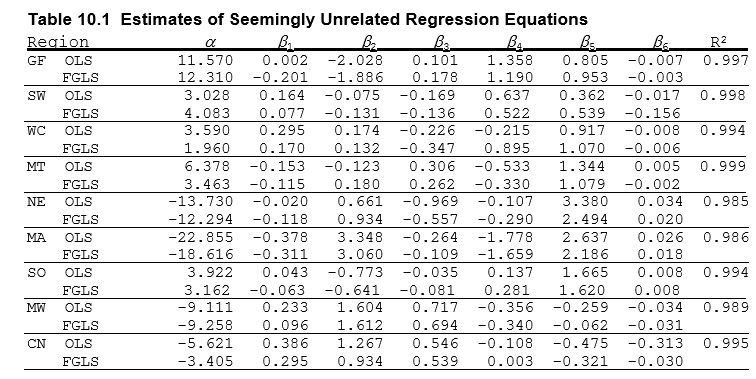
These results can be compared to the results in Greene – they are unsurprisingly identical.
[11]:
display_png(Image("system_correct-greene-table-10-1.png"))
The GLS estimation method requires stronger assumptions for parameter estimates to be consistent. If these are violated then it might be the case that OLS is still consistent (in some sense) and so OLS can be used by passing method="ols" when calling fit.
These results can be compared to Greene”s table – they are identical except the final value which seems to have a small typo.
[12]:
res_ols = mod.fit(method="ols", debiased=True, cov_type="unadjusted")
params = []
r2 = []
for label in res.equation_labels:
    params.append(res_ols.equations[label].params)
    r2.append(res_ols.equations[label].rsquared)
params = pd.concat(params, axis=1)
params.columns = res.equation_labels
params = params.T
params["R2"] = r2
params.style.format("{:0.3f}")
[12]:
| Intercept | lnPC | lnHWY | lnWATER | lnUTIL | lnEMP | UNEMP | R2 | |
|---|---|---|---|---|---|---|---|---|
| GF | 11.567 | 0.002 | -2.029 | 0.101 | 1.358 | 0.805 | -0.007 | 0.997 |
| SW | 3.028 | 0.164 | -0.075 | -0.169 | 0.637 | 0.362 | -0.017 | 0.998 |
| WC | 3.590 | 0.295 | 0.174 | -0.226 | -0.214 | 0.917 | -0.008 | 0.994 |
| MT | 6.378 | -0.153 | -0.123 | 0.306 | -0.533 | 1.344 | 0.005 | 0.999 |
| NE | -13.730 | -0.020 | 0.662 | -0.969 | -0.107 | 3.380 | 0.034 | 0.985 |
| MA | -22.855 | -0.378 | 3.348 | -0.264 | -1.778 | 2.673 | 0.026 | 0.986 |
| SO | 3.927 | 0.043 | -0.773 | -0.035 | 0.140 | 1.665 | 0.008 | 0.994 |
| MW | -9.111 | 0.233 | 1.604 | 0.717 | -0.356 | -0.259 | -0.034 | 0.989 |
| CN | -5.621 | 0.386 | 1.267 | 0.546 | -0.108 | -0.475 | -0.031 | 0.995 |
The parameter estimates for one coefficient – unemployment – can be compared across the two estimation methods.
[13]:
params = pd.concat(
    [
        res_ols.params.iloc[1::7],
        res_ols.std_errors.iloc[1::7],
        res.params.iloc[1::7],
        res.std_errors.iloc[1::7],
    ],
    axis=1,
)
params.columns = ["OLS", "OLS se", "GLS", "GLS se"]
params.index = regions
params
[13]:
| OLS | OLS se | GLS | GLS se | |
|---|---|---|---|---|
| GF | 0.002124 | 0.301235 | -0.200966 | 0.142355 |
| SW | 0.163546 | 0.165995 | 0.076637 | 0.085831 |
| WC | 0.294855 | 0.205417 | 0.169950 | 0.091865 |
| MT | -0.152601 | 0.084031 | -0.114834 | 0.048489 |
| NE | -0.020407 | 0.285621 | 0.118316 | 0.131329 |
| MA | -0.377570 | 0.167307 | -0.310861 | 0.080893 |
| SO | 0.042818 | 0.279472 | -0.063212 | 0.104344 |
| MW | 0.233403 | 0.206248 | 0.095886 | 0.101564 |
| CN | 0.385885 | 0.211083 | 0.294570 | 0.090104 |
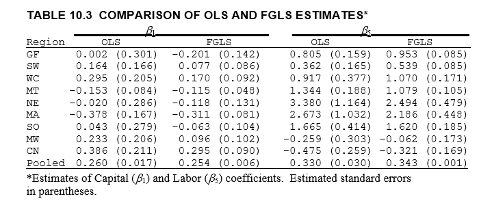
The parameters and their standard errors match those reported in Greene.
[14]:
display_png(Image("system_correct-greene-table-10-3.png"))
Estimation Options
Iterative GLS
These next examples use data on fringe benefits from F. Vella (1993), “A Simple Estimator for Simultaneous Models with Censored Endogenous Regressors” which appears in Wooldridge (2002). The model consists of two equations, one for hourly wage and the other for hourly benefits. The initial model uses the same regressors in both equations.
[15]:
from linearmodels.datasets import fringe

print(fringe.DESCR)
fdata = fringe.load()
F. Vella (1993), "A Simple Estimator for Simultaneous Models with Censored
Endogenous Regressors," International Economic Review 34, 441-457.

annearn                  annual earnings, $
hrearn                   hourly earnings, $
exper                    years work experience
age                      age in years
depends                  number of dependents
married                  =1 if married
tenure                   years with current employer
educ                     years schooling
nrtheast                 =1 if live in northeast
nrthcen                  =1 if live in north central
south                    =1 if live in south
male                     =1 if male
white                    =1 if white
union                    =1 if union member
office                   =1 if office worker
annhrs                   annual hours worked
ind1                     =1 if industry == 1
ind2                     =1 if industry == 2
ind3                     =1 if industry == 3
ind4                     =1 if industry == 4
ind5                     =1 if industry == 5
ind6                     =1 if industry == 6
ind7                     =1 if industry == 7
ind8                     =1 if industry == 8
ind9                     =1 if industry == 9
vacdays                  $ value of vac days
sicklve                  $ value of sick leave
insur                    $ value of employee insur
pension                  $ value of employee pension
annbens                  vacdays+sicklve+insur+pension
hrbens                   hourly benefits, $
annhrssq                 annhrs^2
beratio                  annbens/annearn
lannhrs                  log(annhrs)
tenuresq                 tenure^2
expersq                  exper^2
lannearn                 log(annearn)
peratio                  pension/annearn
vserat                   (vacdays+sicklve)/annearn
The estimated model is reported as “System OLS Estimation” since when all regressors are identical, OLS is used since GLS brings no efficiency gains. OLS will be used when the data structure containing the exogenous regressors in each equations is the same (i.e., id(exog) is the same for all equations).
[16]:
exog = sm.add_constant(
    fdata[
        [
            "educ",
            "exper",
            "expersq",
            "tenure",
            "tenuresq",
            "union",
            "south",
            "nrtheast",
            "nrthcen",
            "married",
            "white",
            "male",
        ]
    ]
)
fmod_data = OrderedDict()
fmod_data["hrearn"] = {"dependent": fdata.hrearn, "exog": exog}
fmod_data["hrbens"] = {"dependent": fdata.hrbens, "exog": exog}
fmod = SUR(fmod_data)
print(fmod.fit(cov_type="unadjusted"))
                           System OLS Estimation Summary
===================================================================================
Estimator:                        OLS   Overall R-squared:                   0.2087
No. Equations.:                     2   McElroy's R-squared:                 0.2926
No. Observations:                 616   Judge's (OLS) R-squared:             0.2087
Date:                Tue, Oct 21 2025   Berndt's R-squared:                  0.4822
Time:                        13:37:42   Dhrymes's R-squared:                 0.2087
                                        Cov. Estimator:                  unadjusted
                                        Num. Constraints:                      None
                 Equation: hrearn, Dependent Variable: hrearn
==============================================================================
            Parameter  Std. Err.     T-stat    P-value    Lower CI    Upper CI
------------------------------------------------------------------------------
const         -2.6321     1.2153    -2.1658     0.0303     -5.0141     -0.2502
educ           0.4588     0.0684     6.7085     0.0000      0.3248      0.5929
exper         -0.0758     0.0567    -1.3367     0.1813     -0.1870      0.0354
expersq        0.0040     0.0012     3.4274     0.0006      0.0017      0.0063
tenure         0.1101     0.0829     1.3276     0.1843     -0.0524      0.2726
tenuresq      -0.0051     0.0032    -1.5640     0.1178     -0.0114      0.0013
union          0.8080     0.4035     2.0026     0.0452      0.0172      1.5988
south         -0.4566     0.5459    -0.8365     0.4029     -1.5265      0.6132
nrtheast      -1.1508     0.5993    -1.9201     0.0548     -2.3254      0.0239
nrthcen       -0.6363     0.5501    -1.1565     0.2475     -1.7145      0.4420
married        0.6424     0.4134     1.5540     0.1202     -0.1678      1.4526
white          1.1409     0.6054     1.8844     0.0595     -0.0458      2.3275
male           1.7847     0.3938     4.5322     0.0000      1.0129      2.5565
                 Equation: hrbens, Dependent Variable: hrbens
==============================================================================
            Parameter  Std. Err.     T-stat    P-value    Lower CI    Upper CI
------------------------------------------------------------------------------
const         -0.8897     0.1453    -6.1225     0.0000     -1.1746     -0.6049
educ           0.0768     0.0082     9.3896     0.0000      0.0608      0.0928
exper          0.0226     0.0068     3.3259     0.0009      0.0093      0.0359
expersq       -0.0005     0.0001    -3.3965     0.0007     -0.0007     -0.0002
tenure         0.0536     0.0099     5.4011     0.0000      0.0341      0.0730
tenuresq      -0.0012     0.0004    -3.0014     0.0027     -0.0019     -0.0004
union          0.3659     0.0482     7.5839     0.0000      0.2713      0.4605
south         -0.0227     0.0653    -0.3476     0.7282     -0.1506      0.1052
nrtheast      -0.0567     0.0717    -0.7918     0.4285     -0.1972      0.0837
nrthcen       -0.0380     0.0658    -0.5776     0.5635     -0.1669      0.0909
married        0.0579     0.0494     1.1706     0.2418     -0.0390      0.1547
white          0.0902     0.0724     1.2453     0.2130     -0.0517      0.2321
male           0.2683     0.0471     5.6985     0.0000      0.1760      0.3606
==============================================================================

Covariance Estimator:
Homoskedastic (Unadjusted) Covariance (Debiased: False, GLS: False)
The estimator can be forced to use GLS by setting method="gls". As can be seen below, the parameter estimates and standard errors do not change even though two-stage GLS is used. The \(R^2\) does change since the left-hand side variable is transformed by the GLS weighting before estimation.
[17]:
print(fmod.fit(method="gls", cov_type="unadjusted"))
                           System GLS Estimation Summary
===================================================================================
Estimator:                        GLS   Overall R-squared:                   0.2087
No. Equations.:                     2   McElroy's R-squared:                 0.2926
No. Observations:                 616   Judge's (OLS) R-squared:             0.2087
Date:                Tue, Oct 21 2025   Berndt's R-squared:                  0.4822
Time:                        13:37:42   Dhrymes's R-squared:                 0.2087
                                        Cov. Estimator:                  unadjusted
                                        Num. Constraints:                      None
                 Equation: hrearn, Dependent Variable: hrearn
==============================================================================
            Parameter  Std. Err.     T-stat    P-value    Lower CI    Upper CI
------------------------------------------------------------------------------
const         -2.6321     1.2153    -2.1658     0.0303     -5.0141     -0.2502
educ           0.4588     0.0684     6.7085     0.0000      0.3248      0.5929
exper         -0.0758     0.0567    -1.3367     0.1813     -0.1870      0.0354
expersq        0.0040     0.0012     3.4274     0.0006      0.0017      0.0063
tenure         0.1101     0.0829     1.3276     0.1843     -0.0524      0.2726
tenuresq      -0.0051     0.0032    -1.5640     0.1178     -0.0114      0.0013
union          0.8080     0.4035     2.0026     0.0452      0.0172      1.5988
south         -0.4566     0.5459    -0.8365     0.4029     -1.5265      0.6132
nrtheast      -1.1508     0.5993    -1.9201     0.0548     -2.3254      0.0239
nrthcen       -0.6363     0.5501    -1.1565     0.2475     -1.7145      0.4420
married        0.6424     0.4134     1.5540     0.1202     -0.1678      1.4526
white          1.1409     0.6054     1.8844     0.0595     -0.0458      2.3275
male           1.7847     0.3938     4.5322     0.0000      1.0129      2.5565
                 Equation: hrbens, Dependent Variable: hrbens
==============================================================================
            Parameter  Std. Err.     T-stat    P-value    Lower CI    Upper CI
------------------------------------------------------------------------------
const         -0.8897     0.1453    -6.1225     0.0000     -1.1746     -0.6049
educ           0.0768     0.0082     9.3896     0.0000      0.0608      0.0928
exper          0.0226     0.0068     3.3259     0.0009      0.0093      0.0359
expersq       -0.0005     0.0001    -3.3965     0.0007     -0.0007     -0.0002
tenure         0.0536     0.0099     5.4011     0.0000      0.0341      0.0730
tenuresq      -0.0012     0.0004    -3.0014     0.0027     -0.0019     -0.0004
union          0.3659     0.0482     7.5839     0.0000      0.2713      0.4605
south         -0.0227     0.0653    -0.3476     0.7282     -0.1506      0.1052
nrtheast      -0.0567     0.0717    -0.7918     0.4285     -0.1972      0.0837
nrthcen       -0.0380     0.0658    -0.5776     0.5635     -0.1669      0.0909
married        0.0579     0.0494     1.1706     0.2418     -0.0390      0.1547
white          0.0902     0.0724     1.2453     0.2130     -0.0517      0.2321
male           0.2683     0.0471     5.6985     0.0000      0.1760      0.3606
==============================================================================

Covariance Estimator:
Homoskedastic (Unadjusted) Covariance (Debiased: False, GLS: True)
The regressors must differ in order to see gains to GLS. Here insignificant variables are dropped from each equation so that the regressors will no longer be identical. The typical standard error is marginally smaller, although this might be due to dropping regressors.
[18]:
exog_earn = sm.add_constant(
    fdata[["educ", "exper", "expersq", "union", "nrtheast", "white"]]
)
exog_bens = sm.add_constant(
    fdata[["educ", "exper", "expersq", "tenure", "tenuresq", "union", "male"]]
)
fmod_data["hrearn"] = {"dependent": fdata.hrearn, "exog": exog_earn}
fmod_data["hrbens"] = {"dependent": fdata.hrbens, "exog": exog_bens}
fmod = SUR(fmod_data)
print(fmod.fit(cov_type="unadjusted"))
                           System GLS Estimation Summary
===================================================================================
Estimator:                        GLS   Overall R-squared:                   0.1685
No. Equations.:                     2   McElroy's R-squared:                 0.2762
No. Observations:                 616   Judge's (OLS) R-squared:             0.1685
Date:                Tue, Oct 21 2025   Berndt's R-squared:                  0.4504
Time:                        13:37:42   Dhrymes's R-squared:                 0.1685
                                        Cov. Estimator:                  unadjusted
                                        Num. Constraints:                      None
                 Equation: hrearn, Dependent Variable: hrearn
==============================================================================
            Parameter  Std. Err.     T-stat    P-value    Lower CI    Upper CI
------------------------------------------------------------------------------
const         -2.5240     1.0857    -2.3246     0.0201     -4.6520     -0.3959
educ           0.5000     0.0685     7.2987     0.0000      0.3657      0.6342
exper         -0.0212     0.0522    -0.4058     0.6849     -0.1234      0.0811
expersq        0.0032     0.0011     2.8776     0.0040      0.0010      0.0055
union          1.1043     0.3928     2.8116     0.0049      0.3345      1.8741
nrtheast      -0.5343     0.4305    -1.2411     0.2146     -1.3780      0.3095
white          1.1320     0.5845     1.9368     0.0528     -0.0136      2.2776
                 Equation: hrbens, Dependent Variable: hrbens
==============================================================================
            Parameter  Std. Err.     T-stat    P-value    Lower CI    Upper CI
------------------------------------------------------------------------------
const         -0.8231     0.1176    -7.0021     0.0000     -1.0535     -0.5927
educ           0.0791     0.0080     9.8927     0.0000      0.0634      0.0948
exper          0.0260     0.0066     3.9114     0.0001      0.0130      0.0390
expersq       -0.0005     0.0001    -3.8469     0.0001     -0.0008     -0.0003
tenure         0.0494     0.0094     5.2409     0.0000      0.0309      0.0679
tenuresq      -0.0010     0.0004    -2.6275     0.0086     -0.0017     -0.0002
union          0.3766     0.0475     7.9259     0.0000      0.2835      0.4698
male           0.2141     0.0433     4.9413     0.0000      0.1292      0.2990
==============================================================================

Covariance Estimator:
Homoskedastic (Unadjusted) Covariance (Debiased: False, GLS: True)
The standard method to estimate models uses two steps. The first uses OLS to estimate the parameters so that the residual covariance can be estimated. The second stage uses the estimated covariance to estimate the model via GLS. Iterative GLS can be used to continue these iterations using the most recent step to estimate the residual covariance and then re-estimating the parameters using GLS. This option can be used by setting iterate=True.
[19]:
fmod_res = fmod.fit(cov_type="unadjusted", iterate=True)
print(fmod_res)
                      System Iterative GLS Estimation Summary
===================================================================================
Estimator:              Iterative GLS   Overall R-squared:                   0.1685
No. Equations.:                     2   McElroy's R-squared:                 0.2749
No. Observations:                 616   Judge's (OLS) R-squared:             0.1685
Date:                Tue, Oct 21 2025   Berndt's R-squared:                  0.4532
Time:                        13:37:42   Dhrymes's R-squared:                 0.1685
                                        Cov. Estimator:                  unadjusted
                                        Num. Constraints:                      None
                 Equation: hrearn, Dependent Variable: hrearn
==============================================================================
            Parameter  Std. Err.     T-stat    P-value    Lower CI    Upper CI
------------------------------------------------------------------------------
const         -2.5147     1.0858    -2.3161     0.0206     -4.6428     -0.3867
educ           0.5001     0.0685     7.3004     0.0000      0.3658      0.6344
exper         -0.0211     0.0522    -0.4044     0.6859     -0.1233      0.0811
expersq        0.0032     0.0011     2.8760     0.0040      0.0010      0.0055
union          1.1043     0.3928     2.8115     0.0049      0.3345      1.8741
nrtheast      -0.5314     0.4305    -1.2342     0.2171     -1.3752      0.3124
white          1.1191     0.5845     1.9145     0.0556     -0.0266      2.2648
                 Equation: hrbens, Dependent Variable: hrbens
==============================================================================
            Parameter  Std. Err.     T-stat    P-value    Lower CI    Upper CI
------------------------------------------------------------------------------
const         -0.8223     0.1176    -6.9947     0.0000     -1.0527     -0.5919
educ           0.0792     0.0080     9.9004     0.0000      0.0635      0.0948
exper          0.0260     0.0066     3.9213     0.0001      0.0130      0.0390
expersq       -0.0005     0.0001    -3.8528     0.0001     -0.0008     -0.0003
tenure         0.0492     0.0094     5.2189     0.0000      0.0307      0.0677
tenuresq      -0.0010     0.0004    -2.6025     0.0093     -0.0017     -0.0002
union          0.3771     0.0475     7.9364     0.0000      0.2840      0.4703
male           0.2107     0.0433     4.8627     0.0000      0.1258      0.2956
==============================================================================

Covariance Estimator:
Homoskedastic (Unadjusted) Covariance (Debiased: False, GLS: True)
The number of GLS iterations can be verified using the iterations attribute of the results.
[20]:
fmod_res.iterations
[20]:
5
Alternative Covariance Estimators
The estimator supports heteroskedasticity robust covariance estimation b setting cov_type="robust". The estimator allows for arbitrary correlation across series with the same time index but not correlation across time periods, which is the same assumption as in the unadjusted estimator. The main difference is that this estimator will correct standard errors for dependence between regressors (or squared regressors) and squared residuals.
Heteroskedasticity Robust Covariance Estimation
In the fringe benefit model there are some large differences between standard errors computed using the the homoskedastic covariance estimator and the heteroskedasticity robust covariance estimator (e.g., exper).
[21]:
fres_het = fmod.fit(cov_type="robust")
print(fres_het.summary)
                           System GLS Estimation Summary
===================================================================================
Estimator:                        GLS   Overall R-squared:                   0.1685
No. Equations.:                     2   McElroy's R-squared:                 0.2762
No. Observations:                 616   Judge's (OLS) R-squared:             0.1685
Date:                Tue, Oct 21 2025   Berndt's R-squared:                  0.4504
Time:                        13:37:42   Dhrymes's R-squared:                 0.1685
                                        Cov. Estimator:                      robust
                                        Num. Constraints:                      None
                 Equation: hrearn, Dependent Variable: hrearn
==============================================================================
            Parameter  Std. Err.     T-stat    P-value    Lower CI    Upper CI
------------------------------------------------------------------------------
const         -2.5240     0.8703    -2.9002     0.0037     -4.2297     -0.8183
educ           0.5000     0.0809     6.1765     0.0000      0.3413      0.6586
exper         -0.0212     0.2270    -0.0932     0.9257     -0.4661      0.4237
expersq        0.0032     0.0059     0.5507     0.5819     -0.0083      0.0148
union          1.1043     0.2857     3.8647     0.0001      0.5443      1.6644
nrtheast      -0.5343     0.5273    -1.0132     0.3110     -1.5678      0.4992
white          1.1320     0.4921     2.3002     0.0214      0.1674      2.0966
                 Equation: hrbens, Dependent Variable: hrbens
==============================================================================
            Parameter  Std. Err.     T-stat    P-value    Lower CI    Upper CI
------------------------------------------------------------------------------
const         -0.8231     0.1082    -7.6087     0.0000     -1.0352     -0.6111
educ           0.0791     0.0081     9.7768     0.0000      0.0632      0.0949
exper          0.0260     0.0059     4.3675     0.0000      0.0143      0.0376
expersq       -0.0005     0.0001    -4.2494     0.0000     -0.0008     -0.0003
tenure         0.0494     0.0097     5.0775     0.0000      0.0303      0.0685
tenuresq      -0.0010     0.0004    -2.4121     0.0159     -0.0018     -0.0002
union          0.3766     0.0514     7.3342     0.0000      0.2760      0.4773
male           0.2141     0.0397     5.3975     0.0000      0.1363      0.2918
==============================================================================

Covariance Estimator:
Heteroskedastic (Robust) Covariance (Debiased: False, GLS: True)
Other supported covariance estimators include "kernel” which implements a HAC and "clustered" which supports 1 and 2-way clustering.
Kernel (HAC)
The supported kernels are "bartlett" (Newey-West), "parzen" (Gallant), and qs (Quadratic Spectral, Andrews). This example uses the Parzen kernel. The kernel’s bandwidth is computed automatically if the parameter bandwidth is not provided.
[22]:
hac_res = fmod.fit(cov_type="kernel", kernel="parzen")
print(hac_res.summary)
                           System GLS Estimation Summary
===================================================================================
Estimator:                        GLS   Overall R-squared:                   0.1685
No. Equations.:                     2   McElroy's R-squared:                 0.2762
No. Observations:                 616   Judge's (OLS) R-squared:             0.1685
Date:                Tue, Oct 21 2025   Berndt's R-squared:                  0.4504
Time:                        13:37:42   Dhrymes's R-squared:                 0.1685
                                        Cov. Estimator:                      kernel
                                        Num. Constraints:                      None
                 Equation: hrearn, Dependent Variable: hrearn
==============================================================================
            Parameter  Std. Err.     T-stat    P-value    Lower CI    Upper CI
------------------------------------------------------------------------------
const         -2.5240     1.0048    -2.5120     0.0120     -4.4933     -0.5547
educ           0.5000     0.0973     5.1391     0.0000      0.3093      0.6907
exper         -0.0212     0.2287    -0.0925     0.9263     -0.4694      0.4270
expersq        0.0032     0.0059     0.5486     0.5833     -0.0084      0.0148
union          1.1043     0.2637     4.1882     0.0000      0.5875      1.6211
nrtheast      -0.5343     0.4800    -1.1131     0.2657     -1.4750      0.4065
white          1.1320     0.4813     2.3520     0.0187      0.1887      2.0753
                 Equation: hrbens, Dependent Variable: hrbens
==============================================================================
            Parameter  Std. Err.     T-stat    P-value    Lower CI    Upper CI
------------------------------------------------------------------------------
const         -0.8231     0.1344    -6.1228     0.0000     -1.0866     -0.5596
educ           0.0791     0.0095     8.3675     0.0000      0.0606      0.0976
exper          0.0260     0.0064     4.0357     0.0001      0.0134      0.0386
expersq       -0.0005     0.0001    -3.9026     0.0001     -0.0008     -0.0003
tenure         0.0494     0.0090     5.5160     0.0000      0.0318      0.0669
tenuresq      -0.0010     0.0003    -2.9161     0.0035     -0.0016     -0.0003
union          0.3766     0.0705     5.3407     0.0000      0.2384      0.5148
male           0.2141     0.0577     3.7117     0.0002      0.1010      0.3271
==============================================================================

Covariance Estimator:
Kernel (HAC) Covariance (Debiased: False, GLS: True, Kernel: parzen)
Clustered (Rogers)
The clustered covariance estimator requires the clusters to be entered as a NumPy array with shape (nobs, 1) or (nobs, 2). This example uses random clusters to illustrate the structure of the group id variable.
[23]:
rs = np.random.RandomState([983476381, 28390328, 23829810])
random_clusters = rs.randint(0, 51, size=(616, 1))
clustered_res = fmod.fit(cov_type="clustered", clusters=random_clusters)
print(clustered_res.summary)
                           System GLS Estimation Summary
===================================================================================
Estimator:                        GLS   Overall R-squared:                   0.1685
No. Equations.:                     2   McElroy's R-squared:                 0.2762
No. Observations:                 616   Judge's (OLS) R-squared:             0.1685
Date:                Tue, Oct 21 2025   Berndt's R-squared:                  0.4504
Time:                        13:37:42   Dhrymes's R-squared:                 0.1685
                                        Cov. Estimator:                   clustered
                                        Num. Constraints:                      None
                 Equation: hrearn, Dependent Variable: hrearn
==============================================================================
            Parameter  Std. Err.     T-stat    P-value    Lower CI    Upper CI
------------------------------------------------------------------------------
const         -2.5240     0.8501    -2.9692     0.0030     -4.1901     -0.8579
educ           0.5000     0.0804     6.2174     0.0000      0.3424      0.6576
exper         -0.0212     0.2285    -0.0926     0.9262     -0.4690      0.4267
expersq        0.0032     0.0059     0.5479     0.5837     -0.0084      0.0149
union          1.1043     0.2696     4.0963     0.0000      0.5759      1.6327
nrtheast      -0.5343     0.5181    -1.0312     0.3024     -1.5497      0.4812
white          1.1320     0.4701     2.4083     0.0160      0.2107      2.0533
                 Equation: hrbens, Dependent Variable: hrbens
==============================================================================
            Parameter  Std. Err.     T-stat    P-value    Lower CI    Upper CI
------------------------------------------------------------------------------
const         -0.8231     0.1077    -7.6435     0.0000     -1.0342     -0.6121
educ           0.0791     0.0080     9.8547     0.0000      0.0634      0.0948
exper          0.0260     0.0059     4.4288     0.0000      0.0145      0.0375
expersq       -0.0005     0.0001    -4.6793     0.0000     -0.0007     -0.0003
tenure         0.0494     0.0105     4.7036     0.0000      0.0288      0.0700
tenuresq      -0.0010     0.0004    -2.2777     0.0227     -0.0018     -0.0001
union          0.3766     0.0525     7.1717     0.0000      0.2737      0.4795
male           0.2141     0.0317     6.7496     0.0000      0.1519      0.2762
==============================================================================

Covariance Estimator:
Heteroskedastic (Robust) Covariance (Debiased: False, GLS: True, Number of Grouping Variables: 1, Number of Groups: 51 (Variable 0), Group Debias: False)
Prespecified Residual Covariance Estimators
The GLS estimator can be used with a user specified covariance. This example uses a covariance where all correlations are identical (equicorrelation) in the state GDP model. The estimator must be used when constructing the model through the sigma keyword argument.
[24]:
avg_corr = (corr - np.eye(9)).mean().mean() * (81 / 72)
rho = np.ones((9, 9)) * avg_corr + (1 - avg_corr) * np.eye(9)
sigma_pre = rho * (std @ std.T)

mod_pre_sigma = SUR(mod_data, sigma=sigma_pre)
res_pre = mod_pre_sigma.fit(cov_type="unadjusted", debiased=True)
print(res_pre.equations["GF"])
                            GLS Estimation Summary
==============================================================================
Eq. Label:                         GF   R-squared:                      0.9966
Dep. Variable:                  lnGSP   Adj. R-squared:                 0.9945
Estimator:                        GLS   Cov. Estimator:             unadjusted
No. Observations:                  17   F-statistic:                    549.95
Date:                Tue, Oct 21 2025   P-value (F-stat)                0.0000
Time:                        13:37:42   Distribution:                  F(6,90)

                             Parameter Estimates
==============================================================================
            Parameter  Std. Err.     T-stat    P-value    Lower CI    Upper CI
------------------------------------------------------------------------------
Intercept      7.9753     4.3819     1.8200     0.0988     -1.7883      17.739
lnPC           0.1011     0.2727     0.3708     0.7185     -0.5065      0.7087
lnHWY         -0.9882     1.0313    -0.9582     0.3606     -3.2862      1.3098
lnWATER        0.0791     0.1134     0.6971     0.5016     -0.1736      0.3318
lnUTIL         0.5160     0.7720     0.6685     0.5190     -1.2040      2.2361
lnEMP          0.8494     0.1426     5.9557     0.0001      0.5316      1.1671
UNEMP         -0.0057     0.0034    -1.6466     0.1307     -0.0134      0.0020

==============================================================================

Covariance Estimator:
Homoskedastic (Unadjusted) Covariance (Debiased: True, GLS: True)
Diagonal Residual Covariance
The default assumption is that there can be arbitrary correlation between series. The model can be estimated assuming no correlation but different variance by setting the keyword argument full_cov=False in the fit method. This is only useful when there are cross-equation parameter restrictions.
Cross-Equation Restrictions
One of the more useful features of using a SUR to estimate a system is the ability to impose constraints on parameters across equations. Here only linear constraints of the form
are supported. Linear constraints are entered by passing a DataFrame with the shape number of constraints by number of parameters. The number and name of parameters can be seen by inspecting the param_names attribute of a model. Below are the parameter names from the state GDP model which consist of the equation label, an underscore, and the variable name. This ensures uniqueness.
[25]:
mod.param_names[:14]
[25]:
['GF_Intercept',
 'GF_lnPC',
 'GF_lnHWY',
 'GF_lnWATER',
 'GF_lnUTIL',
 'GF_lnEMP',
 'GF_UNEMP',
 'SW_Intercept',
 'SW_lnPC',
 'SW_lnHWY',
 'SW_lnWATER',
 'SW_lnUTIL',
 'SW_lnEMP',
 'SW_UNEMP']
The example of a parameter constraint will enforce a common value of the coefficient of unemployment in all equations. This restriction takes the form
where in all examples i is the first series and j is one of the 8 others. In total there are 8 restrictions.
The construction of the restriction array and the non-zero columns are shown below.
[26]:
r = pd.DataFrame(
    columns=mod.param_names,
    index=["rest{0}".format(i) for i in range(8)],
    dtype=np.float64,
)
r.loc[:, :] = 0.0
r.iloc[:, 6] = -1.0
r.iloc[:, 13::7] = np.eye(8)
print(r.iloc[:, 6::7])
       GF_UNEMP  SW_UNEMP  WC_UNEMP  MT_UNEMP  NE_UNEMP  MA_UNEMP  SO_UNEMP  \
rest0      -1.0       1.0       0.0       0.0       0.0       0.0       0.0
rest1      -1.0       0.0       1.0       0.0       0.0       0.0       0.0
rest2      -1.0       0.0       0.0       1.0       0.0       0.0       0.0
rest3      -1.0       0.0       0.0       0.0       1.0       0.0       0.0
rest4      -1.0       0.0       0.0       0.0       0.0       1.0       0.0
rest5      -1.0       0.0       0.0       0.0       0.0       0.0       1.0
rest6      -1.0       0.0       0.0       0.0       0.0       0.0       0.0
rest7      -1.0       0.0       0.0       0.0       0.0       0.0       0.0

       MW_UNEMP  CN_UNEMP
rest0       0.0       0.0
rest1       0.0       0.0
rest2       0.0       0.0
rest3       0.0       0.0
rest4       0.0       0.0
rest5       0.0       0.0
rest6       1.0       0.0
rest7       0.0       1.0
The constraint can be added to an existing model using the add_constraint method. This method requires one input, r and optionally q. if q is not provided, it is set to 0.
Here the constraint is added, the model is estimated, and the parameters for unemployment are displayed. They all have the same value.
[27]:
mod.add_constraints(r)
constrained_res = mod.fit()
constrained_res.params[6::7]
[27]:
GF_UNEMP   -0.005801
SW_UNEMP   -0.005801
WC_UNEMP   -0.005801
MT_UNEMP   -0.005801
NE_UNEMP   -0.005801
MA_UNEMP   -0.005801
SO_UNEMP   -0.005801
MW_UNEMP   -0.005801
CN_UNEMP   -0.005801
Name: params, dtype: float64
Pooling using constraints
More complicated constraints can be used to produce interesting models. Using the same idea as the previous set of constraints, a pooled SUR (excluding the constant) is constructed by restricting all coefficients to have the same value. Here the form of the restriction is
so that the restriction is identical to the previous, only applied to all variables excluding the constant.
Here the estimated from the first two equations are shown. All coefficients except the intercept are identical across equations.
Note: When linear constraints are imposed, the parameter covariance matrix will be singular. Caution is needed to ensure test statistics are meaningful.
[28]:
r2 = np.zeros((8 * 6, r.shape[1]))
loc = 0
for i in range(6):
    for j in range(8):
        r2[loc, i + 1] = -1.0
        r2[loc, 7 * (j + 1) + i + 1] = 1.0
        loc += 1
r2 = pd.DataFrame(r2, columns=mod.param_names)
mod.reset_constraints()
mod.add_constraints(r2)
pooled_res = mod.fit()
print("\n".join(pooled_res.summary.as_text().split("\n")[:33]))
                           System GLS Estimation Summary
===================================================================================
Estimator:                        GLS   Overall R-squared:                   0.9777
No. Equations.:                     9   McElroy's R-squared:                 0.9891
No. Observations:                  17   Judge's (OLS) R-squared:             0.9777
Date:                Tue, Oct 21 2025   Berndt's R-squared:                  0.9974
Time:                        13:37:42   Dhrymes's R-squared:                 0.9777
                                        Cov. Estimator:                      robust
                                        Num. Constraints:                        48
                   Equation: GF, Dependent Variable: lnGSP
==============================================================================
            Parameter  Std. Err.     T-stat    P-value    Lower CI    Upper CI
------------------------------------------------------------------------------
Intercept      0.2732     0.2159     1.2656     0.2057     -0.1499      0.6963
lnPC           0.3639     0.0205     17.763     0.0000      0.3238      0.4041
lnHWY          0.3103     0.0279     11.141     0.0000      0.2557      0.3649
lnWATER        0.0805     0.0109     7.3615     0.0000      0.0591      0.1020
lnUTIL        -0.1733     0.0166    -10.466     0.0000     -0.2057     -0.1408
lnEMP          0.6142     0.0248     24.752     0.0000      0.5655      0.6628
UNEMP         -0.0128     0.0006    -22.939     0.0000     -0.0139     -0.0117
                   Equation: SW, Dependent Variable: lnGSP
==============================================================================
            Parameter  Std. Err.     T-stat    P-value    Lower CI    Upper CI
------------------------------------------------------------------------------
Intercept      0.2869     0.2201     1.3034     0.1924     -0.1445      0.7183
lnPC           0.3639     0.0205     17.763     0.0000      0.3238      0.4041
lnHWY          0.3103     0.0279     11.141     0.0000      0.2557      0.3649
lnWATER        0.0805     0.0109     7.3615     0.0000      0.0591      0.1020
lnUTIL        -0.1733     0.0166    -10.466     0.0000     -0.2057     -0.1408
lnEMP          0.6142     0.0248     24.752     0.0000      0.5655      0.6628
UNEMP         -0.0128     0.0006    -22.939     0.0000     -0.0139     -0.0117
                   Equation: WC, Dependent Variable: lnGSP
==============================================================================
Multivariate OLS
One final feature worth demonstrating is a simple interface for specifying multivariate OLS models. These models have the same regressors and so it is possible to specify them with two arrays. The first is a \(T\) by \(K\) array of dependent variables where each column contains a dependent variable. The second contains the common exogenous regressors.
This example shows how a CAPM can be estimated as a MV OLS.
[29]:
import statsmodels.api as sm
from linearmodels.datasets import french

data = french.load()
factors = sm.add_constant(data[["MktRF"]])
mv_ols = SUR.multivariate_ls(
    data[["S1V1", "S1V3", "S1V5", "S5V1", "S5V3", "S5V5"]], factors
)
mv_ols_res = mv_ols.fit(cov_type="unadjusted")
print(mv_ols_res)
                           System OLS Estimation Summary
===================================================================================
Estimator:                        OLS   Overall R-squared:                   0.6564
No. Equations.:                     6   McElroy's R-squared:                 0.8776
No. Observations:                 819   Judge's (OLS) R-squared:             0.6564
Date:                Tue, Oct 21 2025   Berndt's R-squared:                  0.9773
Time:                        13:37:43   Dhrymes's R-squared:                 0.6564
                                        Cov. Estimator:                  unadjusted
                                        Num. Constraints:                      None
                   Equation: S1V1, Dependent Variable: S1V1
==============================================================================
            Parameter  Std. Err.     T-stat    P-value    Lower CI    Upper CI
------------------------------------------------------------------------------
const         -0.0020     0.0017    -1.1608     0.2457     -0.0054      0.0014
MktRF          1.3736     0.0403     34.101     0.0000      1.2947      1.4526
                   Equation: S1V3, Dependent Variable: S1V3
==============================================================================
            Parameter  Std. Err.     T-stat    P-value    Lower CI    Upper CI
------------------------------------------------------------------------------
const          0.0048     0.0012     4.0973     0.0000      0.0025      0.0072
MktRF          1.0711     0.0276     38.879     0.0000      1.0171      1.1251
                   Equation: S1V5, Dependent Variable: S1V5
==============================================================================
            Parameter  Std. Err.     T-stat    P-value    Lower CI    Upper CI
------------------------------------------------------------------------------
const          0.0082     0.0013     6.5142     0.0000      0.0057      0.0106
MktRF          1.0538     0.0293     36.019     0.0000      0.9965      1.1111
                   Equation: S5V1, Dependent Variable: S5V1
==============================================================================
            Parameter  Std. Err.     T-stat    P-value    Lower CI    Upper CI
------------------------------------------------------------------------------
const          0.0032     0.0005     5.8787     0.0000      0.0021      0.0042
MktRF          0.9861     0.0126     78.376     0.0000      0.9615      1.0108
                   Equation: S5V3, Dependent Variable: S5V3
==============================================================================
            Parameter  Std. Err.     T-stat    P-value    Lower CI    Upper CI
------------------------------------------------------------------------------
const          0.0052     0.0007     7.4953     0.0000      0.0039      0.0066
MktRF          0.8472     0.0162     52.204     0.0000      0.8154      0.8790
                   Equation: S5V5, Dependent Variable: S5V5
==============================================================================
            Parameter  Std. Err.     T-stat    P-value    Lower CI    Upper CI
------------------------------------------------------------------------------
const          0.0051     0.0011     4.5167     0.0000      0.0029      0.0073
MktRF          0.9851     0.0263     37.515     0.0000      0.9337      1.0366
==============================================================================

Covariance Estimator:
Homoskedastic (Unadjusted) Covariance (Debiased: False, GLS: False)
Using GLS with common regressors
As noted previously, forcing GLS has no effect (except on changing the \(R^2\)). This can be seen below.
[30]:
print(mv_ols.fit(cov_type="unadjusted", method="gls"))
                           System GLS Estimation Summary
===================================================================================
Estimator:                        GLS   Overall R-squared:                   0.6564
No. Equations.:                     6   McElroy's R-squared:                 0.8776
No. Observations:                 819   Judge's (OLS) R-squared:             0.6564
Date:                Tue, Oct 21 2025   Berndt's R-squared:                  0.9773
Time:                        13:37:43   Dhrymes's R-squared:                 0.6564
                                        Cov. Estimator:                  unadjusted
                                        Num. Constraints:                      None
                   Equation: S1V1, Dependent Variable: S1V1
==============================================================================
            Parameter  Std. Err.     T-stat    P-value    Lower CI    Upper CI
------------------------------------------------------------------------------
const         -0.0020     0.0017    -1.1608     0.2457     -0.0054      0.0014
MktRF          1.3736     0.0403     34.101     0.0000      1.2947      1.4526
                   Equation: S1V3, Dependent Variable: S1V3
==============================================================================
            Parameter  Std. Err.     T-stat    P-value    Lower CI    Upper CI
------------------------------------------------------------------------------
const          0.0048     0.0012     4.0973     0.0000      0.0025      0.0072
MktRF          1.0711     0.0276     38.879     0.0000      1.0171      1.1251
                   Equation: S1V5, Dependent Variable: S1V5
==============================================================================
            Parameter  Std. Err.     T-stat    P-value    Lower CI    Upper CI
------------------------------------------------------------------------------
const          0.0082     0.0013     6.5142     0.0000      0.0057      0.0106
MktRF          1.0538     0.0293     36.019     0.0000      0.9965      1.1111
                   Equation: S5V1, Dependent Variable: S5V1
==============================================================================
            Parameter  Std. Err.     T-stat    P-value    Lower CI    Upper CI
------------------------------------------------------------------------------
const          0.0032     0.0005     5.8787     0.0000      0.0021      0.0042
MktRF          0.9861     0.0126     78.376     0.0000      0.9615      1.0108
                   Equation: S5V3, Dependent Variable: S5V3
==============================================================================
            Parameter  Std. Err.     T-stat    P-value    Lower CI    Upper CI
------------------------------------------------------------------------------
const          0.0052     0.0007     7.4953     0.0000      0.0039      0.0066
MktRF          0.8472     0.0162     52.204     0.0000      0.8154      0.8790
                   Equation: S5V5, Dependent Variable: S5V5
==============================================================================
            Parameter  Std. Err.     T-stat    P-value    Lower CI    Upper CI
------------------------------------------------------------------------------
const          0.0051     0.0011     4.5167     0.0000      0.0029      0.0073
MktRF          0.9851     0.0263     37.515     0.0000      0.9337      1.0366
==============================================================================

Covariance Estimator:
Homoskedastic (Unadjusted) Covariance (Debiased: False, GLS: True)