Cointegration Testing
This setup code is required to run in an IPython notebook
[1]:
import warnings
warnings.simplefilter('ignore')

%matplotlib inline
import matplotlib.pyplot as plt
import seaborn

seaborn.set_style('darkgrid')
plt.rc("figure", figsize=(16, 6))
plt.rc("savefig", dpi=90)
plt.rc("font",family="sans-serif")
plt.rc("font",size=14)
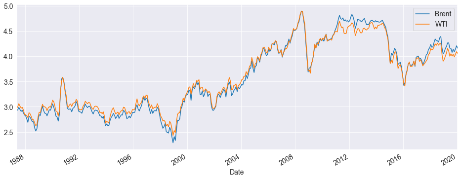
We will look at the spot prices of crude oil measured in Cushing, OK for West Texas Intermediate Crude, and Brent Crude. The underlying data in this data set come from the U.S. Energy Information Administration.
[2]:
from arch.data import crude
import numpy as np
data = crude.load()
log_price = np.log(data)

ax = log_price.plot()
xl = ax.set_xlim(log_price.index.min(), log_price.index.max())
We can verify these both of these series appear to contains unit roots using Augmented Dickey-Fuller tests. The p-values are large indicating that the null cannot be rejected.
[3]:
from arch.unitroot import ADF

ADF(log_price.WTI, trend="c")
[3]:
| Test Statistic | -1.780 |
| P-value | 0.391 |
| Lags | 1 |
Trend: Constant
Critical Values: -3.45 (1%), -2.87 (5%), -2.57 (10%)
Null Hypothesis: The process contains a unit root.
Alternative Hypothesis: The process is weakly stationary.
[4]:
ADF(log_price.Brent, trend="c")
[4]:
| Test Statistic | -1.655 |
| P-value | 0.454 |
| Lags | 1 |
Trend: Constant
Critical Values: -3.45 (1%), -2.87 (5%), -2.57 (10%)
Null Hypothesis: The process contains a unit root.
Alternative Hypothesis: The process is weakly stationary.
The Engle-Granger test is a 2-step test that first estimates a cross-sectional regression, and then tests the residuals from this regression using an Augmented Dickey-Fuller distribution with modified critical values. The cross-sectional regression is
where \(Y_t\) and \(X_t\) combine to contain the set of variables being tested for cointegration and \(D_t\) are a set of deterministic regressors that might include a constant, a time trend, or a quadratic time trend. The trend is specified using trend as
"n": No trend"c": Constant"ct": Constant and time trend"ctt": Constant, time and quadratic trends
Here we assume that that cointegrating relationship is exact so that no deterministics are needed.
[5]:
from arch.unitroot import engle_granger

eg_test = engle_granger(log_price.WTI, log_price.Brent, trend="n")
eg_test
[5]:
| Test Statistic | -3.468 |
| P-value | 0.007 |
| ADF Lag length | 0 |
| Estimated Root ρ (γ+1) | 0.939 |
Trend: Constant
Critical Values: -2.47 (10%), -2.78 (5%), -3.37 (1%)
Null Hypothesis: No Cointegration
Alternative Hypothesis: Cointegration
Distribution Order: 1
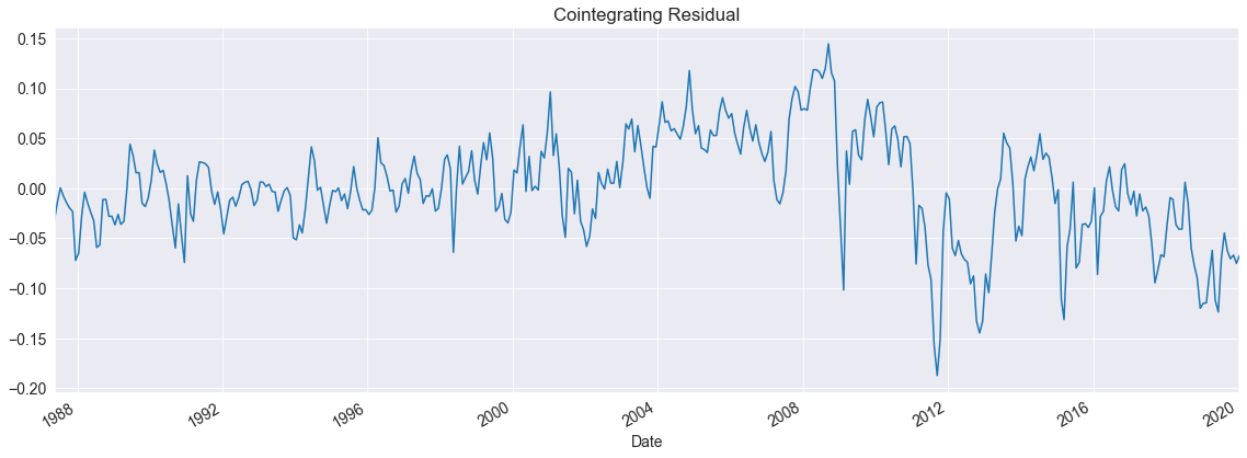
The plot method can be used to plot the model residual. We see that while this appears to be mean 0, it might have a trend in it.
[6]:
fig = eg_test.plot()
The estimated cointegrating vector is exposed through he cointegrating_vector property. Here we see it is very close to \([1, -1]\), indicating a simple no-arbitrage relationship.
[7]:
eg_test.cointegrating_vector
[7]:
WTI      1.000000
Brent   -1.000621
dtype: float64
We can rerun the test with both a constant and a time trend to see how this affects the conclusion. We firmly reject the null of no cointegration even with this alternative assumption.
[8]:
eg_test = engle_granger(log_price.WTI, log_price.Brent, trend="ct")
eg_test
[8]:
| Test Statistic | -5.837 |
| P-value | 0.000 |
| ADF Lag length | 0 |
| Estimated Root ρ (γ+1) | 0.840 |
Trend: Constant
Critical Values: -3.52 (10%), -3.81 (5%), -4.37 (1%)
Null Hypothesis: No Cointegration
Alternative Hypothesis: Cointegration
Distribution Order: 1
[9]:
eg_test.cointegrating_vector
[9]:
WTI      1.000000
Brent   -0.931769
const   -0.296939
trend    0.000185
dtype: float64
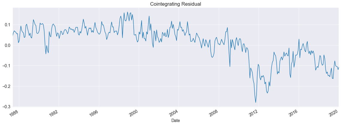
The residuals are clearly mean zero but show evidence of a structural break around the financial crisis of 2008.
[10]:
fig = eg_test.plot()

To investigate the changes in the 2008 financial crisis, we can re-run the test on only the pre-crisis period.
[11]:
eg_test = engle_granger(log_price[:"2008"].WTI, log_price[:"2008"].Brent, trend="n")
eg_test
[11]:
| Test Statistic | -4.962 |
| P-value | 0.000 |
| ADF Lag length | 0 |
| Estimated Root ρ (γ+1) | 0.825 |
Trend: Constant
Critical Values: -2.48 (10%), -2.79 (5%), -3.38 (1%)
Null Hypothesis: No Cointegration
Alternative Hypothesis: Cointegration
Distribution Order: 1
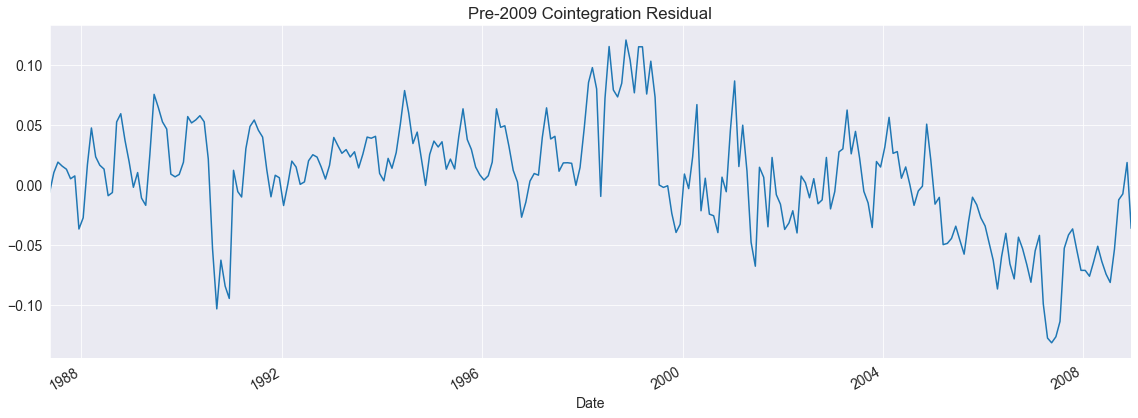
These residuals look quite a bit better although it is possible the break in the cointegrating vector happened around 2005 when oil prices first surged.
[12]:
fig = eg_test.plot()
ax = fig.get_axes()[0]
title = ax.set_title("Pre-2009 Cointegration Residual")
Phillips-Ouliaris
The Phillips-Ouliaris tests consists four distinct tests. Two are similar to the Engle-Granger test, only using a Phillips & Perron-like approach replaces the lags in the ADF test with a long-run variance estimator. The other two use variance-ratio like approaches to test. In both cases the test stabilizes when there is no cointegration and diverges due to singularity of the covariance matrix of the I(1) time series when there is cointegration.
\(Z_t\) - Like PP using the t-stat of the AR(1) coefficient in an AR(1) of the residual from the cross-sectional regression.
\(Z_\alpha\) - Like PP using \(T(\alpha-1)\) and a bias term from the same AR(1)
\(P_u\) - A univariate variance ratio test.
\(P_z\) - A multivariate variance ratio test.
The four test statistics all agree on the crude oil data.
The \(Z_t\) and \(Z_\alpha\) test statistics are both based on the quantity \(\gamma=\rho-1\) from the regression \(y_t = d_t \Delta + \rho y_{t-1} + \epsilon_t\). The null is rejected in favor of the alternative when \(\gamma<0\) so that the test statistic is below its critical value.
[13]:
from arch.unitroot.cointegration import phillips_ouliaris

po_zt_test = phillips_ouliaris(log_price.WTI, log_price.Brent, trend="c", test_type="Zt")
po_zt_test.summary()
[13]:
| Test Statistic | -5.357 |
| P-value | 0.000 |
| Kernel | Bartlett |
| Bandwidth | 10.185 |
Trend: Constant
Critical Values: -3.06 (10%), -3.36 (5%), -3.94 (1%)
Null Hypothesis: No Cointegration
Alternative Hypothesis: Cointegration
Distribution Order: 3
[14]:
po_za_test = phillips_ouliaris(log_price.WTI, log_price.Brent, trend="c", test_type="Za")
po_za_test.summary()
[14]:
| Test Statistic | -53.531 |
| P-value | 0.000 |
| Kernel | Bartlett |
| Bandwidth | 10.185 |
Trend: Constant
Critical Values: -16.95 (10%), -20.34 (5%), -27.77 (1%)
Null Hypothesis: No Cointegration
Alternative Hypothesis: Cointegration
Distribution Order: 3
The \(P_u\) and \(P_z\) statistics are variance ratios where under the null the numerator and denominator are balanced and so converge at the same rate. Under the alternative the denominstor convreges to zero and the statistic diverges, so that rejection of the null occcurs when the test statistic is above a critical value.
[15]:
po_pu_test = phillips_ouliaris(log_price.WTI, log_price.Brent, trend="c", test_type="Pu")
po_pu_test.summary()
[15]:
| Test Statistic | 102.868 |
| P-value | 0.000 |
| Kernel | Bartlett |
| Bandwidth | 14.648 |
Trend: Constant
Critical Values: 27.02 (10%), 32.94 (5%), 46.02 (1%)
Null Hypothesis: No Cointegration
Alternative Hypothesis: Cointegration
Distribution Order: 2
[16]:
po_pu_test = phillips_ouliaris(log_price.WTI, log_price.Brent, trend="c", test_type="Pz")
po_pu_test.summary()
[16]:
| Test Statistic | 114.601 |
| P-value | 0.000 |
| Kernel | Bartlett |
| Bandwidth | 14.648 |
Trend: Constant
Critical Values: 45.40 (10%), 52.41 (5%), 67.37 (1%)
Null Hypothesis: No Cointegration
Alternative Hypothesis: Cointegration
Distribution Order: 2
The cointegrating residual is identical to the EG test since the first step is identical.
[17]:
fig = po_zt_test.plot()