ARCH Modeling¶

This setup code is required to run in an IPython notebook

[1]:

import matplotlib.pyplot as plt
import seaborn

seaborn.set_style("darkgrid")
plt.rc("figure", figsize=(16, 6))
plt.rc("savefig", dpi=90)
plt.rc("font", family="sans-serif")
plt.rc("font", size=14)

Setup¶

These examples will all make use of financial data from Yahoo! Finance. This data set can be loaded from arch.data.sp500.

[2]:

import datetime as dt

import arch.data.sp500

st = dt.datetime(1988, 1, 1)
en = dt.datetime(2018, 1, 1)
data = arch.data.sp500.load()
market = data["Adj Close"]
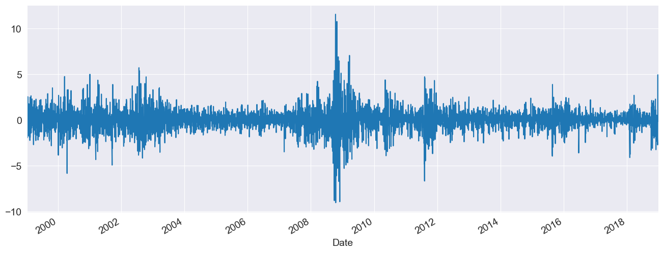
returns = 100 * market.pct_change().dropna()
ax = returns.plot()
xlim = ax.set_xlim(returns.index.min(), returns.index.max())

../_images/univariate_univariate_volatility_modeling_5_0.png

Specifying Common Models¶

The simplest way to specify a model is to use the model constructor arch.arch_model which can specify most common models. The simplest invocation of arch will return a model with a constant mean, GARCH(1,1) volatility process and normally distributed errors.

\[r_t = \mu + \epsilon_t\]

\[\sigma^2_t = \omega + \alpha \epsilon_{t-1}^2 + \beta \sigma_{t-1}^2\]

\[\epsilon_t = \sigma_t e_t,\,\,\, e_t \sim N(0,1)\]

The model is estimated by calling fit. The optional inputs iter controls the frequency of output form the optimizer, and disp controls whether convergence information is returned. The results class returned offers direct access to the estimated parameters and related quantities, as well as a summary of the estimation results.

GARCH (with a Constant Mean)¶

The default set of options produces a model with a constant mean, GARCH(1,1) conditional variance and normal errors.

[3]:

from arch import arch_model

am = arch_model(returns)
res = am.fit(update_freq=5)
print(res.summary())

Iteration:      5,   Func. Count:     35,   Neg. LLF: 6970.2765831170655
Iteration:     10,   Func. Count:     63,   Neg. LLF: 6936.718477482658
Optimization terminated successfully    (Exit mode 0)
            Current function value: 6936.718476988985
            Iterations: 11
            Function evaluations: 68
            Gradient evaluations: 11
                     Constant Mean - GARCH Model Results
==============================================================================
Dep. Variable:              Adj Close   R-squared:                       0.000
Mean Model:             Constant Mean   Adj. R-squared:                  0.000
Vol Model:                      GARCH   Log-Likelihood:               -6936.72
Distribution:                  Normal   AIC:                           13881.4
Method:            Maximum Likelihood   BIC:                           13907.5
                                        No. Observations:                 5030
Date:                Mon, Nov 04 2024   Df Residuals:                     5029
Time:                        16:00:46   Df Model:                            1
                                 Mean Model
============================================================================
                 coef    std err          t      P>|t|      95.0% Conf. Int.
----------------------------------------------------------------------------
mu             0.0564  1.149e-02      4.906  9.302e-07 [3.384e-02,7.887e-02]
                              Volatility Model
============================================================================
                 coef    std err          t      P>|t|      95.0% Conf. Int.
----------------------------------------------------------------------------
omega          0.0175  4.683e-03      3.738  1.854e-04 [8.328e-03,2.669e-02]
alpha[1]       0.1022  1.301e-02      7.852  4.105e-15   [7.665e-02,  0.128]
beta[1]        0.8852  1.380e-02     64.125      0.000     [  0.858,  0.912]
============================================================================

Covariance estimator: robust

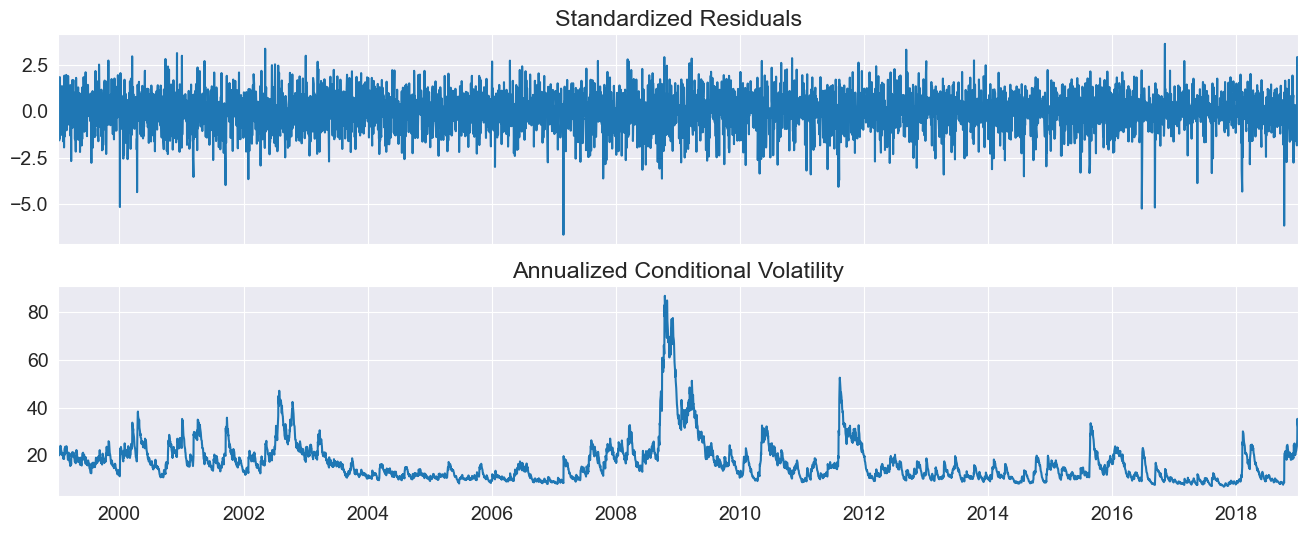
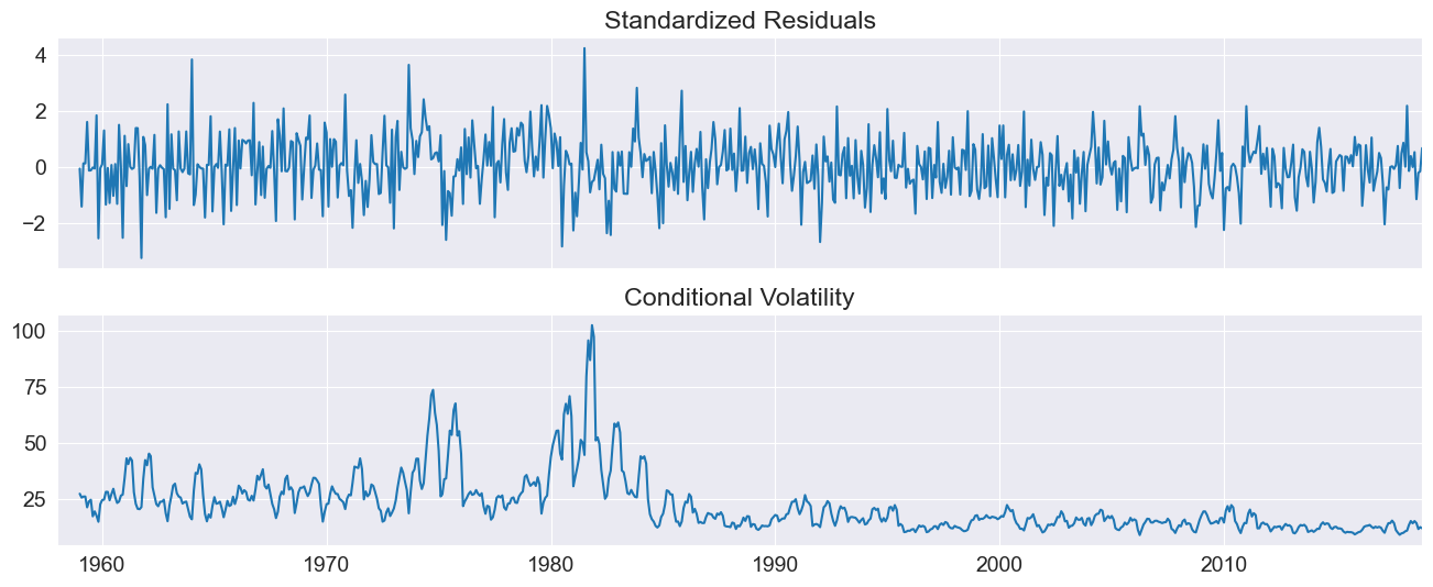
plot() can be used to quickly visualize the standardized residuals and conditional volatility.

[4]:

fig = res.plot(annualize="D")

../_images/univariate_univariate_volatility_modeling_12_0.png

GJR-GARCH¶

Additional inputs can be used to construct other models. This example sets o to 1, which includes one lag of an asymmetric shock which transforms a GARCH model into a GJR-GARCH model with variance dynamics given by

\[\sigma^2_t = \omega + \alpha \epsilon_{t-1}^2 + \gamma \epsilon_{t-1}^2 I_{[\epsilon_{t-1}<0]}+ \beta \sigma_{t-1}^2\]

where \(I\) is an indicator function that takes the value 1 when its argument is true.

The log likelihood improves substantially with the introduction of an asymmetric term, and the parameter estimate is highly significant.

[5]:

am = arch_model(returns, p=1, o=1, q=1)
res = am.fit(update_freq=5, disp="off")
print(res.summary())

                   Constant Mean - GJR-GARCH Model Results
==============================================================================
Dep. Variable:              Adj Close   R-squared:                       0.000
Mean Model:             Constant Mean   Adj. R-squared:                  0.000
Vol Model:                  GJR-GARCH   Log-Likelihood:               -6822.88
Distribution:                  Normal   AIC:                           13655.8
Method:            Maximum Likelihood   BIC:                           13688.4
                                        No. Observations:                 5030
Date:                Mon, Nov 04 2024   Df Residuals:                     5029
Time:                        16:00:47   Df Model:                            1
                                  Mean Model
=============================================================================
                 coef    std err          t      P>|t|       95.0% Conf. Int.
-----------------------------------------------------------------------------
mu             0.0175  1.145e-02      1.529      0.126 [-4.936e-03,3.995e-02]
                               Volatility Model
=============================================================================
                 coef    std err          t      P>|t|       95.0% Conf. Int.
-----------------------------------------------------------------------------
omega          0.0196  4.051e-03      4.830  1.362e-06  [1.163e-02,2.751e-02]
alpha[1]   2.2928e-10  1.026e-02  2.234e-08      1.000 [-2.011e-02,2.011e-02]
gamma[1]       0.1831  2.266e-02      8.079  6.543e-16      [  0.139,  0.227]
beta[1]        0.8922  1.458e-02     61.200      0.000      [  0.864,  0.921]
=============================================================================

Covariance estimator: robust

TARCH/ZARCH¶

TARCH (also known as ZARCH) model the volatility using absolute values. This model is specified using power=1.0 since the default power, 2, corresponds to variance processes that evolve in squares.

The volatility process in a TARCH model is given by

\[\sigma_t = \omega + \alpha \left|\epsilon_{t-1}\right| + \gamma \left|\epsilon_{t-1}\right| I_{[\epsilon_{t-1}<0]}+ \beta \sigma_{t-1}\]

More general models with other powers (\(\kappa\)) have volatility dynamics given by

\[\sigma_t^\kappa = \omega + \alpha \left|\epsilon_{t-1}\right|^\kappa + \gamma \left|\epsilon_{t-1}\right|^\kappa I_{[\epsilon_{t-1}<0]}+ \beta \sigma_{t-1}^\kappa\]

where the conditional variance is \(\left(\sigma_t^\kappa\right)^{2/\kappa}\).

The TARCH model also improves the fit, although the change in the log likelihood is less dramatic.

[6]:

am = arch_model(returns, p=1, o=1, q=1, power=1.0)
res = am.fit(update_freq=5)
print(res.summary())

Iteration:      5,   Func. Count:     45,   Neg. LLF: 6829.203002130782
Iteration:     10,   Func. Count:     79,   Neg. LLF: 6799.178617397159
Optimization terminated successfully    (Exit mode 0)
            Current function value: 6799.178521515934
            Iterations: 13
            Function evaluations: 96
            Gradient evaluations: 13
                  Constant Mean - TARCH/ZARCH Model Results
==============================================================================
Dep. Variable:              Adj Close   R-squared:                       0.000
Mean Model:             Constant Mean   Adj. R-squared:                  0.000
Vol Model:                TARCH/ZARCH   Log-Likelihood:               -6799.18
Distribution:                  Normal   AIC:                           13608.4
Method:            Maximum Likelihood   BIC:                           13641.0
                                        No. Observations:                 5030
Date:                Mon, Nov 04 2024   Df Residuals:                     5029
Time:                        16:00:47   Df Model:                            1
                                  Mean Model
=============================================================================
                 coef    std err          t      P>|t|       95.0% Conf. Int.
-----------------------------------------------------------------------------
mu             0.0143  1.091e-02      1.311      0.190 [-7.087e-03,3.570e-02]
                               Volatility Model
=============================================================================
                 coef    std err          t      P>|t|       95.0% Conf. Int.
-----------------------------------------------------------------------------
omega          0.0258  4.100e-03      6.299  2.990e-10  [1.779e-02,3.386e-02]
alpha[1]       0.0000  9.156e-03      0.000      1.000 [-1.794e-02,1.794e-02]
gamma[1]       0.1707  1.601e-02     10.664  1.505e-26      [  0.139,  0.202]
beta[1]        0.9098  9.672e-03     94.066      0.000      [  0.891,  0.929]
=============================================================================

Covariance estimator: robust

Student’s T Errors¶

Financial returns are often heavy tailed, and a Student’s T distribution is a simple method to capture this feature. The call to arch changes the distribution from a Normal to a Students’s T.

The standardized residuals appear to be heavy tailed with an estimated degree of freedom near 10. The log-likelihood also shows a large increase.

[7]:

am = arch_model(returns, p=1, o=1, q=1, power=1.0, dist="StudentsT")
res = am.fit(update_freq=5)
print(res.summary())

Iteration:      5,   Func. Count:     50,   Neg. LLF: 6728.995165345449
Iteration:     10,   Func. Count:     90,   Neg. LLF: 6722.151187114983
Optimization terminated successfully    (Exit mode 0)
            Current function value: 6722.1511835327055
            Iterations: 14
            Function evaluations: 117
            Gradient evaluations: 13
                     Constant Mean - TARCH/ZARCH Model Results
====================================================================================
Dep. Variable:                    Adj Close   R-squared:                       0.000
Mean Model:                   Constant Mean   Adj. R-squared:                  0.000
Vol Model:                      TARCH/ZARCH   Log-Likelihood:               -6722.15
Distribution:      Standardized Student's t   AIC:                           13456.3
Method:                  Maximum Likelihood   BIC:                           13495.4
                                              No. Observations:                 5030
Date:                      Mon, Nov 04 2024   Df Residuals:                     5029
Time:                              16:00:47   Df Model:                            1
                                 Mean Model
============================================================================
                 coef    std err          t      P>|t|      95.0% Conf. Int.
----------------------------------------------------------------------------
mu             0.0323  2.132e-03     15.137  9.241e-52 [2.809e-02,3.644e-02]
                               Volatility Model
=============================================================================
                 coef    std err          t      P>|t|       95.0% Conf. Int.
-----------------------------------------------------------------------------
omega          0.0201  3.490e-03      5.748  9.021e-09  [1.322e-02,2.690e-02]
alpha[1]       0.0000  8.222e-03      0.000      1.000 [-1.612e-02,1.612e-02]
gamma[1]       0.1721  1.512e-02     11.388  4.817e-30      [  0.143,  0.202]
beta[1]        0.9139  9.578e-03     95.415      0.000      [  0.895,  0.933]
                              Distribution
========================================================================
                 coef    std err          t      P>|t|  95.0% Conf. Int.
------------------------------------------------------------------------
nu             7.9549      0.880      9.037  1.605e-19 [  6.230,  9.680]
========================================================================

Covariance estimator: robust

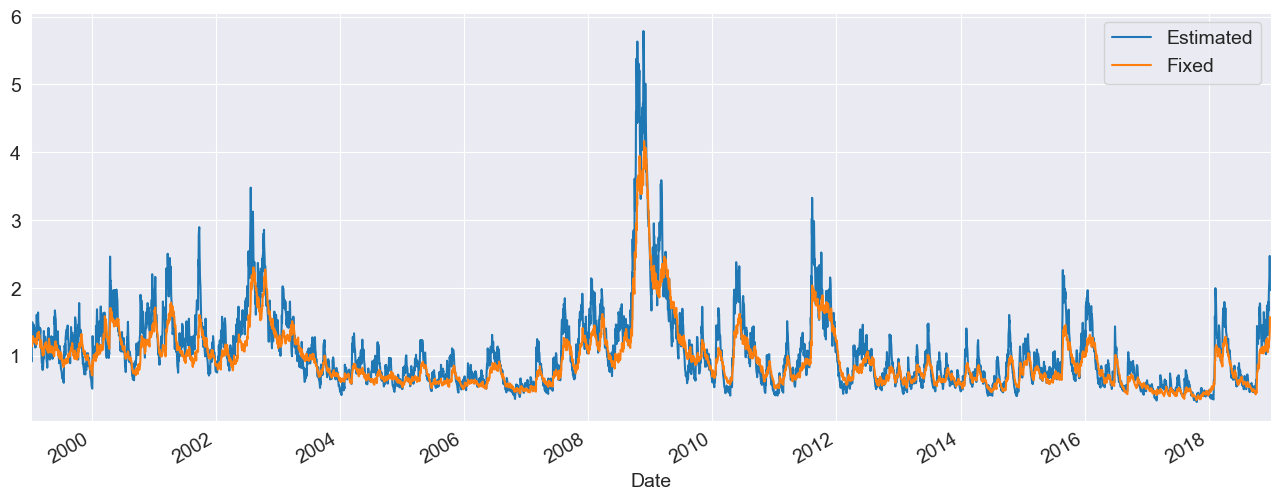
Fixing Parameters¶

In some circumstances, fixed rather than estimated parameters might be of interest. A model-result-like class can be generated using the fix() method. The class returned is identical to the usual model result class except that information about inference (standard errors, t-stats, etc) is not available.

In the example, I fix the parameters to a symmetric version of the previously estimated model.

[8]:

fixed_res = am.fix([0.0235, 0.01, 0.06, 0.0, 0.9382, 8.0])
print(fixed_res.summary())

                      Constant Mean - TARCH/ZARCH Model Results
=====================================================================================
Dep. Variable:                     Adj Close   R-squared:                          --
Mean Model:                    Constant Mean   Adj. R-squared:                     --
Vol Model:                       TARCH/ZARCH   Log-Likelihood:               -6908.93
Distribution:       Standardized Student's t   AIC:                           13829.9
Method:            User-specified Parameters   BIC:                           13869.0
                                               No. Observations:                 5030
Date:                       Mon, Nov 04 2024
Time:                               16:00:47
      Mean Model
=====================
                 coef
---------------------
mu             0.0235
   Volatility Model
=====================
                 coef
---------------------
omega          0.0100
alpha[1]       0.0600
gamma[1]       0.0000
beta[1]        0.9382
     Distribution
=====================
                 coef
---------------------
nu             8.0000
=====================

Results generated with user-specified parameters.
Std. errors not available when the model is not estimated,

[9]:

import pandas as pd

df = pd.concat([res.conditional_volatility, fixed_res.conditional_volatility], axis=1)
df.columns = ["Estimated", "Fixed"]
subplot = df.plot()
subplot.set_xlim(xlim)

[9]:

(np.float64(10596.0), np.float64(17896.0))

../_images/univariate_univariate_volatility_modeling_24_1.png

Building a Model From Components¶

Models can also be systematically assembled from the three model components:

A mean model (arch.mean)
- Zero mean (ZeroMean) - useful if using residuals from a model estimated separately
- Constant mean (ConstantMean) - common for most liquid financial assets
- Autoregressive (ARX) with optional exogenous regressors
- Heterogeneous (HARX) autoregression with optional exogenous regressors
- Exogenous regressors only (LS)
A volatility process (arch.volatility)
- ARCH (ARCH)
- GARCH (GARCH)
- GJR-GARCH (GARCH using o argument)
- TARCH/ZARCH (GARCH using power argument set to 1)
- Power GARCH and Asymmetric Power GARCH (GARCH using power)
- Exponentially Weighted Moving Average Variance with estimated coefficient (EWMAVariance)
- Heterogeneous ARCH (HARCH)
- Parameterless Models
  - Exponentially Weighted Moving Average Variance, known as RiskMetrics (EWMAVariance)
  - Weighted averages of EWMAs, known as the RiskMetrics 2006 methodology (RiskMetrics2006)
A distribution (arch.distribution)
- Normal (Normal)
- Standardized Students’s T (StudentsT)

Mean Models¶

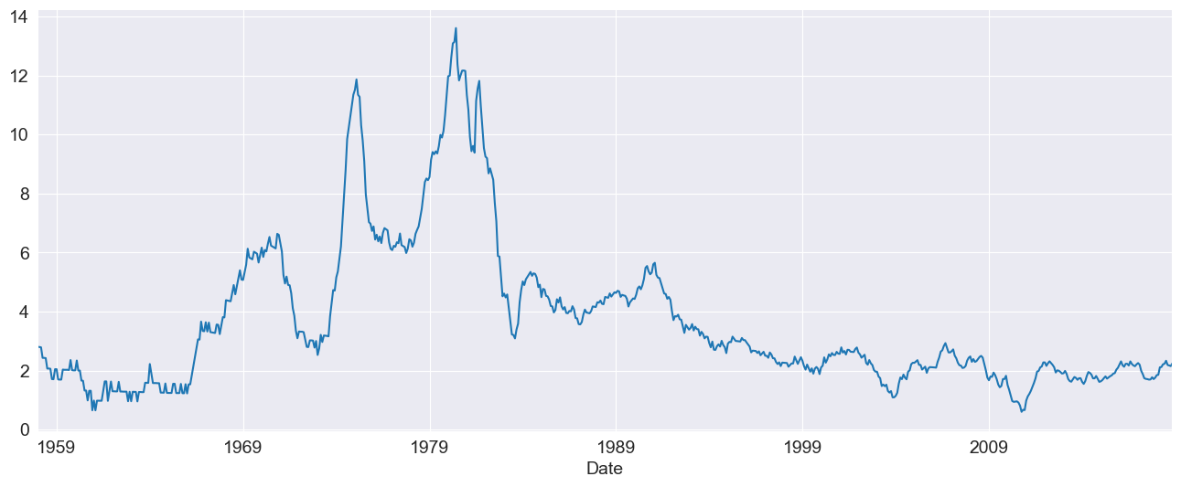
The first choice is the mean model. For many liquid financial assets, a constant mean (or even zero) is adequate. For other series, such as inflation, a more complicated model may be required. These examples make use of Core CPI downloaded from the Federal Reserve Economic Data site.

[10]:

import arch.data.core_cpi

core_cpi = arch.data.core_cpi.load()
ann_inflation = 100 * core_cpi.CPILFESL.pct_change(12).dropna()
fig = ann_inflation.plot()

../_images/univariate_univariate_volatility_modeling_29_0.png

All mean models are initialized with constant variance and normal errors. For ARX models, the lags argument specifies the lags to include in the model.

[11]:

from arch.univariate import ARX

ar = ARX(100 * ann_inflation, lags=[1, 3, 12])
print(ar.fit().summary())

                     AR - Constant Variance Model Results
==============================================================================
Dep. Variable:               CPILFESL   R-squared:                       0.991
Mean Model:                        AR   Adj. R-squared:                  0.991
Vol Model:          Constant Variance   Log-Likelihood:               -3299.84
Distribution:                  Normal   AIC:                           6609.68
Method:            Maximum Likelihood   BIC:                           6632.57
                                        No. Observations:                  719
Date:                Mon, Nov 04 2024   Df Residuals:                      715
Time:                        16:00:48   Df Model:                            4
                                   Mean Model
===============================================================================
                   coef    std err          t      P>|t|       95.0% Conf. Int.
-------------------------------------------------------------------------------
Const            4.0216      2.030      1.981  4.762e-02    [4.218e-02,  8.001]
CPILFESL[1]      1.1921  3.475e-02     34.306 6.315e-258      [  1.124,  1.260]
CPILFESL[3]     -0.1798  4.076e-02     -4.411  1.030e-05   [ -0.260,-9.989e-02]
CPILFESL[12]    -0.0232  1.370e-02     -1.692  9.058e-02 [-5.002e-02,3.666e-03]
                              Volatility Model
============================================================================
                 coef    std err          t      P>|t|      95.0% Conf. Int.
----------------------------------------------------------------------------
sigma2       567.4180     64.487      8.799  1.381e-18 [4.410e+02,6.938e+02]
============================================================================

Covariance estimator: White's Heteroskedasticity Consistent Estimator

Volatility Processes¶

Volatility processes can be added a a mean model using the volatility property. This example adds an ARCH(5) process to model volatility. The arguments iter and disp are used in fit() to suppress estimation output.

[12]:

from arch.univariate import ARCH, GARCH

ar.volatility = ARCH(p=5)
res = ar.fit(update_freq=0, disp="off")
print(res.summary())

                           AR - ARCH Model Results
==============================================================================
Dep. Variable:               CPILFESL   R-squared:                       0.991
Mean Model:                        AR   Adj. R-squared:                  0.991
Vol Model:                       ARCH   Log-Likelihood:               -3174.60
Distribution:                  Normal   AIC:                           6369.19
Method:            Maximum Likelihood   BIC:                           6414.97
                                        No. Observations:                  719
Date:                Mon, Nov 04 2024   Df Residuals:                      715
Time:                        16:00:48   Df Model:                            4
                                   Mean Model
===============================================================================
                   coef    std err          t      P>|t|       95.0% Conf. Int.
-------------------------------------------------------------------------------
Const            2.8500      1.883      1.513      0.130      [ -0.841,  6.541]
CPILFESL[1]      1.0859  3.534e-02     30.726 2.593e-207      [  1.017,  1.155]
CPILFESL[3]     -0.0788  3.855e-02     -2.045  4.084e-02   [ -0.154,-3.282e-03]
CPILFESL[12]    -0.0189  1.157e-02     -1.630      0.103 [-4.154e-02,3.820e-03]
                             Volatility Model
==========================================================================
                 coef    std err          t      P>|t|    95.0% Conf. Int.
--------------------------------------------------------------------------
omega         76.8648     16.016      4.799  1.592e-06 [ 45.475,1.083e+02]
alpha[1]       0.1345  4.003e-02      3.359  7.826e-04 [5.600e-02,  0.213]
alpha[2]       0.2280  6.284e-02      3.628  2.860e-04   [  0.105,  0.351]
alpha[3]       0.1838  6.802e-02      2.702  6.893e-03 [5.047e-02,  0.317]
alpha[4]       0.2538  7.826e-02      3.242  1.185e-03   [  0.100,  0.407]
alpha[5]       0.1954  7.091e-02      2.756  5.855e-03 [5.644e-02,  0.334]
==========================================================================

Covariance estimator: robust

Plotting the standardized residuals and the conditional volatility shows some large (in magnitude) errors, even when standardized.

[13]:

fig = res.plot()

../_images/univariate_univariate_volatility_modeling_36_0.png

Distributions¶

Finally the distribution can be changed from the default normal to a standardized Student’s T using the distribution property of a mean model.

The Student’s t distribution improves the model, and the degree of freedom is estimated to be near 8.

[14]:

from arch.univariate import StudentsT

ar.distribution = StudentsT()
res = ar.fit(update_freq=0, disp="off")
print(res.summary())

                              AR - ARCH Model Results
====================================================================================
Dep. Variable:                     CPILFESL   R-squared:                       0.991
Mean Model:                              AR   Adj. R-squared:                  0.991
Vol Model:                             ARCH   Log-Likelihood:               -3168.25
Distribution:      Standardized Student's t   AIC:                           6358.51
Method:                  Maximum Likelihood   BIC:                           6408.86
                                              No. Observations:                  719
Date:                      Mon, Nov 04 2024   Df Residuals:                      715
Time:                              16:00:49   Df Model:                            4
                                   Mean Model
===============================================================================
                   coef    std err          t      P>|t|       95.0% Conf. Int.
-------------------------------------------------------------------------------
Const            3.1219      1.861      1.678  9.344e-02      [ -0.526,  6.769]
CPILFESL[1]      1.0843  3.525e-02     30.763 8.300e-208      [  1.015,  1.153]
CPILFESL[3]     -0.0730  3.873e-02     -1.885  5.948e-02    [ -0.149,2.918e-03]
CPILFESL[12]    -0.0236  1.316e-02     -1.791  7.333e-02 [-4.934e-02,2.226e-03]
                             Volatility Model
==========================================================================
                 coef    std err          t      P>|t|    95.0% Conf. Int.
--------------------------------------------------------------------------
omega         87.3417     20.621      4.235  2.280e-05 [ 46.925,1.278e+02]
alpha[1]       0.1715  5.063e-02      3.386  7.086e-04 [7.222e-02,  0.271]
alpha[2]       0.2202  6.394e-02      3.444  5.741e-04 [9.486e-02,  0.345]
alpha[3]       0.1547  6.327e-02      2.446  1.446e-02 [3.073e-02,  0.279]
alpha[4]       0.2117  7.288e-02      2.905  3.675e-03 [6.885e-02,  0.355]
alpha[5]       0.1959  7.853e-02      2.495  1.260e-02 [4.200e-02,  0.350]
                              Distribution
========================================================================
                 coef    std err          t      P>|t|  95.0% Conf. Int.
------------------------------------------------------------------------
nu             9.0465      3.367      2.687  7.220e-03 [  2.447, 15.646]
========================================================================

Covariance estimator: robust

WTI Crude¶

The next example uses West Texas Intermediate Crude data from FRED. Three models are fit using alternative distributional assumptions. The results are printed, where we can see that the normal has a much lower log-likelihood than either the Standard Student’s T or the Standardized Skew Student’s T – however, these two are fairly close. The closeness of the T and the Skew T indicate that returns are not heavily skewed.

[15]:

from collections import OrderedDict

import arch.data.wti

crude = arch.data.wti.load()
crude_ret = 100 * crude.DCOILWTICO.dropna().pct_change().dropna()
res_normal = arch_model(crude_ret).fit(disp="off")
res_t = arch_model(crude_ret, dist="t").fit(disp="off")
res_skewt = arch_model(crude_ret, dist="skewt").fit(disp="off")
lls = pd.Series(
    OrderedDict(
        (
            ("normal", res_normal.loglikelihood),
            ("t", res_t.loglikelihood),
            ("skewt", res_skewt.loglikelihood),
        )
    )
)
print(lls)
params = pd.DataFrame(
    OrderedDict(
        (
            ("normal", res_normal.params),
            ("t", res_t.params),
            ("skewt", res_skewt.params),
        )
    )
)
params

normal   -18165.858870
t        -17919.643916
skewt    -17916.669052
dtype: float64

[15]:

	normal	t	skewt
alpha[1]	0.085627	0.064980	0.064889
beta[1]	0.909098	0.927950	0.928215
eta	NaN	NaN	6.186541
lambda	NaN	NaN	-0.036986
mu	0.046682	0.056438	0.040928
nu	NaN	6.178598	NaN
omega	0.055806	0.048516	0.047683

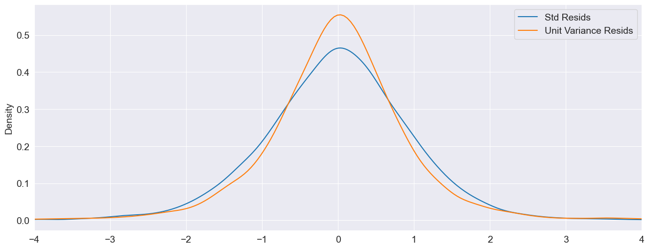
The standardized residuals can be computed by dividing the residuals by the conditional volatility. These are plotted along with the (unstandardized, but scaled) residuals. The non-standardized residuals are more peaked in the center indicating that the distribution is somewhat more heavy tailed than that of the standardized residuals.

[16]:

std_resid = res_normal.resid / res_normal.conditional_volatility
unit_var_resid = res_normal.resid / res_normal.resid.std()
df = pd.concat([std_resid, unit_var_resid], axis=1)
df.columns = ["Std Resids", "Unit Variance Resids"]
subplot = df.plot(kind="kde", xlim=(-4, 4))

../_images/univariate_univariate_volatility_modeling_44_0.png

Simulation¶

All mean models expose a method to simulate returns from assuming the model is correctly specified. There are two required parameters, params which are the model parameters, and nobs, the number of observations to produce.

Below we simulate from a GJR-GARCH(1,1) with Skew-t errors using parameters estimated on the WTI series. The simulation returns a DataFrame with 3 columns:

data: The simulated data, which includes any mean dynamics.
volatility: The conditional volatility series
errors: The simulated errors generated to produce the model. The errors are the difference between the data and its conditional mean, and can be transformed into the standardized errors by dividing by the volatility.

[17]:

res = arch_model(crude_ret, p=1, o=1, q=1, dist="skewt").fit(disp="off")
pd.DataFrame(res.params)

[17]:

	params
mu	0.029365
omega	0.044374
alpha[1]	0.044344
gamma[1]	0.036104
beta[1]	0.931280
eta	6.211281
lambda	-0.041616

[18]:

sim_mod = arch_model(None, p=1, o=1, q=1, dist="skewt")

sim_data = sim_mod.simulate(res.params, 1000)
sim_data.head()

[18]:

	data	volatility	errors
0	-0.288481	3.636821	-0.317846
1	3.067474	3.517108	3.038109
2	2.262375	3.460297	2.233010
3	6.831472	3.378803	6.802107
4	-3.469485	3.567618	-3.498851

Simulations can be reproduced using a NumPy RandomState. This requires constructing a model from components where the RandomState instance is passed into to the distribution when the model is created.

The cell below contains code that builds a model with a constant mean, GJR-GARCH volatility and Skew \(t\) errors initialized with a user-provided RandomState. Saving the initial state allows it to be restored later so that the simulation can be run with the same random values.

[19]:

import numpy as np

from arch.univariate import ConstantMean, SkewStudent

rs = np.random.RandomState([892380934, 189201902, 129129894, 9890437])
# Save the initial state to reset later
state = rs.get_state()

dist = SkewStudent(seed=rs)
vol = GARCH(p=1, o=1, q=1)
repro_mod = ConstantMean(None, volatility=vol, distribution=dist)

repro_mod.simulate(res.params, 1000).head()

[19]:

	data	volatility	errors
0	1.616836	4.787697	1.587470
1	4.106780	4.637129	4.077415
2	4.530200	4.561457	4.500834
3	2.284833	4.507739	2.255468
4	3.378519	4.381016	3.349153

Resetting the state using set_state shows that calling simulate using the same underlying state in the RandomState produces the same objects.

[20]:

# Reset the state to the initial state
rs.set_state(state)
repro_mod.simulate(res.params, 1000).head()

[20]:

	data	volatility	errors
0	1.616836	4.787697	1.587470
1	4.106780	4.637129	4.077415
2	4.530200	4.561457	4.500834
3	2.284833	4.507739	2.255468
4	3.378519	4.381016	3.349153