Volatility Scenarios
Custom random-number generators can be used to implement scenarios where shock follow a particular pattern. For example, suppose you wanted to find out what would happen if there were 5 days of shocks that were larger than average. In most circumstances, the shocks in a GARCH model have unit variance. This could be changed so that the first 5 shocks have variance 4, or twice the standard deviation.
Another scenario would be to over sample a specific period for the shocks. When using the standard bootstrap method (filtered historical simulation) the shocks are drawn using iid sampling from the history. While this approach is standard and well-grounded, it might be desirable to sample from a specific period. This can be implemented using a custom random number generator. This strategy is precisely how the filtered historical simulation is implemented internally, only where the draws are uniformly sampled from the entire history.
First, some preliminaries
[1]:
from __future__ import annotations

import matplotlib.pyplot as plt
import numpy as np
import pandas as pd
import seaborn as sns
from arch.univariate import GARCH, ConstantMean, Normal

sns.set_style("darkgrid")
plt.rc("figure", figsize=(16, 6))
plt.rc("savefig", dpi=90)
plt.rc("font", family="sans-serif")
plt.rc("font", size=14)
This example makes use of returns from the NASDAQ index. The scenario bootstrap will make use of returns in the run-up to and during the Financial Crisis of 2008.
[2]:
import arch.data.nasdaq

data = arch.data.nasdaq.load()
nasdaq = data["Adj Close"]
print(nasdaq.head())
Date
1999-01-04    2208.050049
1999-01-05    2251.270020
1999-01-06    2320.860107
1999-01-07    2326.090088
1999-01-08    2344.409912
Name: Adj Close, dtype: float64
Next, the returns are computed and the model is constructed. The model is constructed from the building blocks. It is a standard model and could have been (almost) equivalently constructed using
mod = arch_model(rets, mean='constant', p=1, o=1, q=1)
The one advantage of constructing the model using the components is that the NumPy RandomState that is used to simulate from the model can be externally set. This allows the generator seed to be easily set and for the state to reset, if needed.
NOTE: It is always a good idea to scale return by 100 before estimating ARCH-type models. This helps the optimizer converse since the scale of the volatility intercept is much closer to the scale of the other parameters in the model.
[3]:
rets = 100 * nasdaq.pct_change().dropna()

# Build components to set the state for the distribution
random_state = np.random.RandomState(1)
dist = Normal(seed=random_state)
volatility = GARCH(1, 1, 1)

mod = ConstantMean(rets, volatility=volatility, distribution=dist)
Fitting the model is standard.
[4]:
res = mod.fit(disp="off")
res
[4]:
                   Constant Mean - GJR-GARCH Model Results
==============================================================================
Dep. Variable:              Adj Close   R-squared:                       0.000
Mean Model:             Constant Mean   Adj. R-squared:                  0.000
Vol Model:                  GJR-GARCH   Log-Likelihood:               -8196.75
Distribution:                  Normal   AIC:                           16403.5
Method:            Maximum Likelihood   BIC:                           16436.1
                                        No. Observations:                 5030
Date:                Tue, Oct 21 2025   Df Residuals:                     5029
Time:                        08:39:48   Df Model:                            1
                                 Mean Model
============================================================================
                 coef    std err          t      P>|t|      95.0% Conf. Int.
----------------------------------------------------------------------------
mu             0.0376  1.476e-02      2.549  1.081e-02 [8.693e-03,6.656e-02]
                               Volatility Model
=============================================================================
                 coef    std err          t      P>|t|       95.0% Conf. Int.
-----------------------------------------------------------------------------
omega          0.0214  5.001e-03      4.281  1.861e-05  [1.161e-02,3.121e-02]
alpha[1]       0.0152  8.442e-03      1.802  7.148e-02 [-1.330e-03,3.176e-02]
gamma[1]       0.1265  2.024e-02      6.250  4.109e-10    [8.684e-02,  0.166]
beta[1]        0.9100  1.107e-02     82.232      0.000      [  0.888,  0.932]
=============================================================================

Covariance estimator: robust
ARCHModelResult, id: 0x7f1f76ac0ad0
GJR-GARCH models support analytical forecasts, which is the default. The forecasts are produced for all of 2017 using the estimated model parameters.
All GARCH specification are complete models in the sense that they specify a distribution. This allows simulations to be produced using the assumptions in the model. The forecast function can be made to produce simulations using the assumed distribution by setting method='simulation'.
These forecasts are similar to the analytical forecasts above. As the number of simulation increases towards \(\infty\), the simulation-based forecasts will converge to the analytical values above.
[5]:
sim_forecasts = res.forecast(start="1-1-2017", method="simulation", horizon=10)
print(sim_forecasts.residual_variance.dropna().head())
                h.01      h.02      h.03      h.04      h.05      h.06  \
Date
2017-01-03  0.623295  0.637251  0.647817  0.663746  0.673404  0.687952
2017-01-04  0.599455  0.617539  0.635838  0.649695  0.659733  0.667267
2017-01-05  0.567297  0.583415  0.597571  0.613065  0.621790  0.636180
2017-01-06  0.542506  0.555688  0.570280  0.585426  0.595551  0.608487
2017-01-09  0.515452  0.528771  0.542658  0.559684  0.580434  0.594855

                h.07      h.08      h.09      h.10
Date
2017-01-03  0.697221  0.707707  0.717701  0.729465
2017-01-04  0.686503  0.699708  0.707203  0.718560
2017-01-05  0.650287  0.663344  0.679835  0.692300
2017-01-06  0.619195  0.638180  0.653185  0.661366
2017-01-09  0.605136  0.621835  0.634091  0.653222
Custom Random Generators
forecast supports replacing the generator based on the assumed distribution of residuals in the model with any other generator. A shock generator should usually produce unit variance shocks. However, in this example the first 5 shocks generated have variance 2, and the remainder are standard normal. This scenario consists of a period of consistently surprising volatility where the volatility has shifted for some reason.
The forecast variances are much larger and grow faster than those from either method previously illustrated. This reflects the increase in volatility in the first 5 days.
[6]:
forecasts = res.forecast(start="1-1-2017", horizon=10)
print(forecasts.residual_variance.dropna().head())
                h.01      h.02      h.03      h.04      h.05      h.06  \
Date
2017-01-03  0.623295  0.637504  0.651549  0.665431  0.679154  0.692717
2017-01-04  0.599455  0.613940  0.628257  0.642408  0.656397  0.670223
2017-01-05  0.567297  0.582153  0.596837  0.611352  0.625699  0.639880
2017-01-06  0.542506  0.557649  0.572616  0.587410  0.602034  0.616488
2017-01-09  0.515452  0.530906  0.546183  0.561282  0.576208  0.590961

                h.07      h.08      h.09      h.10
Date
2017-01-03  0.706124  0.719376  0.732475  0.745423
2017-01-04  0.683890  0.697399  0.710752  0.723950
2017-01-05  0.653897  0.667753  0.681448  0.694985
2017-01-06  0.630776  0.644899  0.658858  0.672656
2017-01-09  0.605543  0.619957  0.634205  0.648288
[7]:
import numpy as np

random_state = np.random.RandomState(1)


def scenario_rng(
    size: tuple[int, int],
) -> np.ndarray[tuple[int, int], np.dtype[np.float64]]:
    shocks = random_state.standard_normal(size)
    shocks[:, :5] *= np.sqrt(2)
    return shocks


scenario_forecasts = res.forecast(
    start="1-1-2017", method="simulation", horizon=10, rng=scenario_rng
)
print(scenario_forecasts.residual_variance.dropna().head())
                h.01      h.02      h.03      h.04      h.05      h.06  \
Date
2017-01-03  0.623295  0.685911  0.745202  0.821112  0.886289  0.966737
2017-01-04  0.599455  0.668181  0.743119  0.811486  0.877539  0.936587
2017-01-05  0.567297  0.629195  0.691225  0.758891  0.816663  0.893986
2017-01-06  0.542506  0.596301  0.656603  0.721505  0.778286  0.849680
2017-01-09  0.515452  0.567086  0.622224  0.689831  0.775048  0.845656

                h.07      h.08      h.09      h.10
Date
2017-01-03  0.970796  0.977504  0.982202  0.992547
2017-01-04  0.955295  0.965540  0.966432  0.974248
2017-01-05  0.905952  0.915208  0.930777  0.938636
2017-01-06  0.856175  0.873865  0.886221  0.890002
2017-01-09  0.851104  0.864591  0.874696  0.894397
Bootstrap Scenarios
forecast supports Filtered Historical Simulation (FHS) using method='bootstrap'. This is effectively a simulation method where the simulated shocks are generated using iid sampling from the history of the demeaned and standardized return data. Custom bootstraps are another application of rng. Here an object is used to hold the shocks. This object exposes a method (rng) the acts like a random number generator, except that it only returns values that were provided in the shocks
parameter.
The internal implementation of the FHS uses a method almost identical to this where shocks contain the entire history.
[8]:
class ScenarioBootstrapRNG:
    def __init__(
        self,
        shocks: np.ndarray[tuple[int], np.dtype[np.float64]],
        random_state: np.random.RandomState,
    ) -> None:
        self._shocks = np.array(shocks, dtype=float).squeeze()  # 1d
        self._rs = random_state
        self.n = shocks.shape[0]

    def rng(self, size: int) -> np.ndarray[tuple[int], np.dtype[np.float64]]:
        idx = self._rs.randint(0, self.n, size=size)
        return self._shocks[idx]


random_state = np.random.RandomState(1)
std_shocks = res.resid / res.conditional_volatility
shocks = std_shocks["2008-08-01":"2008-11-10"]
scenario_bootstrap = ScenarioBootstrapRNG(shocks, random_state)
bs_forecasts = res.forecast(
    start="1-1-2017", method="simulation", horizon=10, rng=scenario_bootstrap.rng
)
print(bs_forecasts.residual_variance.dropna().head())
                h.01      h.02      h.03      h.04      h.05      h.06  \
Date
2017-01-03  0.623295  0.676081  0.734322  0.779325  0.828189  0.898202
2017-01-04  0.599455  0.645237  0.697133  0.750169  0.816280  0.888417
2017-01-05  0.567297  0.610493  0.665995  0.722954  0.777860  0.840369
2017-01-06  0.542506  0.597387  0.644534  0.691387  0.741206  0.783319
2017-01-09  0.515452  0.561312  0.611026  0.647824  0.700559  0.757398

                h.07      h.08      h.09      h.10
Date
2017-01-03  0.958215  1.043704  1.124684  1.203893
2017-01-04  0.945120  1.013400  1.084042  1.158148
2017-01-05  0.889032  0.961424  1.022413  1.097192
2017-01-06  0.840667  0.895559  0.957266  1.019497
2017-01-09  0.820788  0.887791  0.938708  1.028614
Visualizing the differences
The final forecast values are used to illustrate how these are different. The analytical and standard simulation are virtually identical. The simulated scenario grows rapidly for the first 5 periods and then more slowly. The bootstrap scenario grows quickly and consistently due to the magnitude of the shocks in the financial crisis.
[9]:
df = pd.concat(
    [
        forecasts.residual_variance.iloc[-1],
        sim_forecasts.residual_variance.iloc[-1],
        scenario_forecasts.residual_variance.iloc[-1],
        bs_forecasts.residual_variance.iloc[-1],
    ],
    axis=1,
)
df.columns = ["Analytic", "Simulation", "Scenario Sim", "Bootstrp Scenario"]
# Plot annualized vol
subplot = np.sqrt(252 * df).plot(legend=False)
legend = subplot.legend(frameon=False)
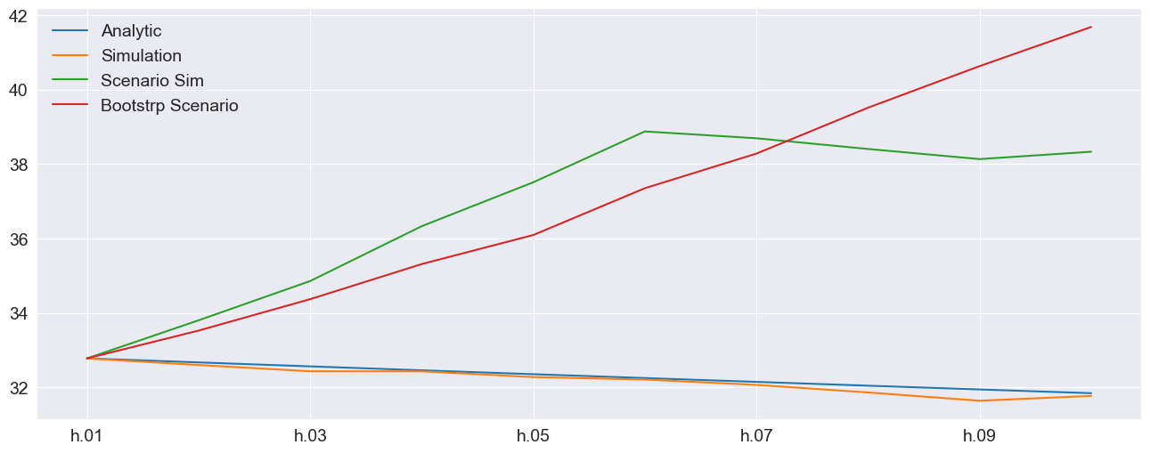
[10]:
subplot = np.sqrt(252 * df).plot
Comparing the paths
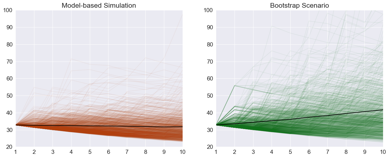
The paths are available on the attribute simulations. Plotting the paths shows important differences between the two scenarios beyond the average differences plotted above. Both start at the same point.
[11]:
fig, axes = plt.subplots(1, 2)
colors = sns.color_palette("dark")
# The paths for the final observation
sim_paths = sim_forecasts.simulations.residual_variances[-1].T
bs_paths = bs_forecasts.simulations.residual_variances[-1].T

x = np.arange(1, 11)
# Plot the paths and the mean, set the axis to have the same limit
axes[0].plot(x, np.sqrt(252 * sim_paths), color=colors[1], alpha=0.05)
axes[0].plot(
    x, np.sqrt(252 * sim_forecasts.residual_variance.iloc[-1]), color="k", alpha=1
)
axes[0].set_title("Model-based Simulation")
axes[0].set_xticks(np.arange(1, 11))
axes[0].set_xlim(1, 10)
axes[0].set_ylim(20, 100)

axes[1].plot(x, np.sqrt(252 * bs_paths), color=colors[2], alpha=0.05)
axes[1].plot(
    x, np.sqrt(252 * bs_forecasts.residual_variance.iloc[-1]), color="k", alpha=1
)
axes[1].set_xticks(np.arange(1, 11))
axes[1].set_xlim(1, 10)
axes[1].set_ylim(20, 100)
title = axes[1].set_title("Bootstrap Scenario")
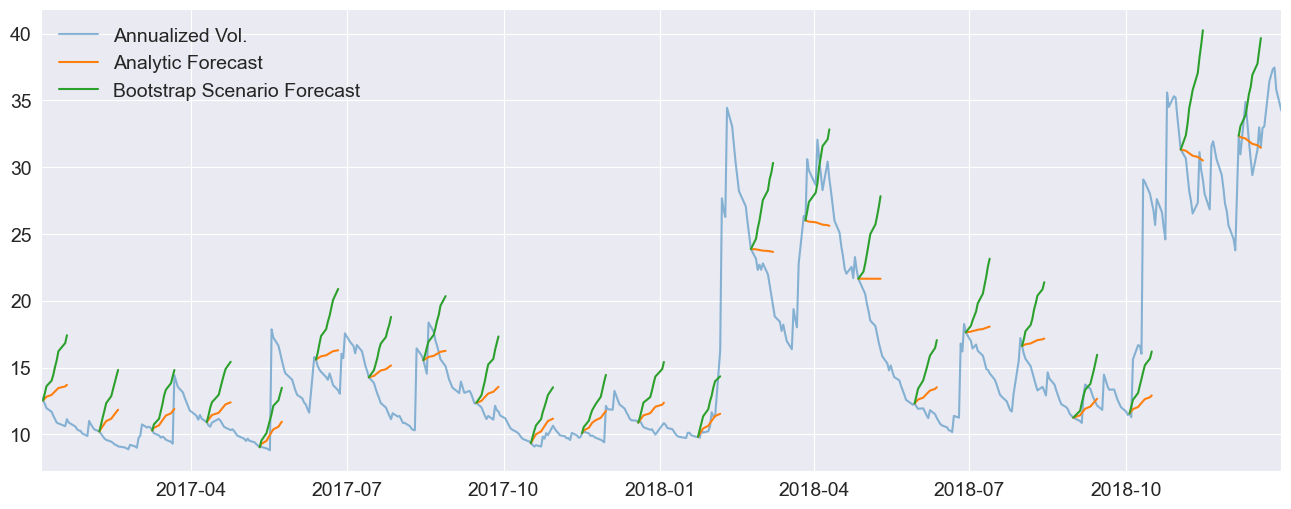
Comparing across the year
A hedgehog plot is useful for showing the differences between the two forecasting methods across the year, instead of a single day.
[12]:
analytic = forecasts.residual_variance.dropna()
bs = bs_forecasts.residual_variance.dropna()
fig, ax = plt.subplots(1, 1)
vol = res.conditional_volatility["2017-1-1":"2019-1-1"]
idx = vol.index
ax.plot(np.sqrt(252) * vol, alpha=0.5)
colors = sns.color_palette()
for i in range(0, len(vol), 22):
    a = analytic.iloc[i]
    b = bs.iloc[i]
    loc = idx.get_loc(a.name)
    new_idx = idx[loc + 1 : loc + 11]
    a.index = new_idx
    b.index = new_idx
    ax.plot(np.sqrt(252 * a), color=colors[1])
    ax.plot(np.sqrt(252 * b), color=colors[2])
labels = ["Annualized Vol.", "Analytic Forecast", "Bootstrap Scenario Forecast"]
legend = ax.legend(labels, frameon=False)
xlim = ax.set_xlim(vol.index[0], vol.index[-1])